Important Words

Setup

Loading Libraries

library(tidyverse)
library(tidytext)
library(gutenbergr)
library(geomtextpath)

if(!require(wordcloud2)){
  install.packages("wordcloud2")
  library(wordcloud2)
}

Setting up Frankenstein

frank <- gutenberg_download(84)

frankenstein |> 
  unnest_tokens(
    word,
    text,
    token = "words"
  ) |> 
  mutate(
    word = str_remove_all(word, "_")
  ) |> 
  separate_wider_delim(
    section, 
    delim = " ", 
    names = c("prefix", "number")
  ) |> 
  mutate(number = as.numeric(number))-> 
  frank_tokens

frank |> 
  mutate(                
    text = str_squish(text),
    section = case_when(
      str_detect(text, "^Letter \\d+$") ~ text,
      str_detect(text, "^Chapter \\d+$") ~ text
    )
  ) |>             
  fill(section) |>
  filter(text != section,
         !is.na(section),
         str_length(text) > 0) |>
  mutate(line_number = row_number()) ->
  frankenstein

What are the most frequent words in each chapter?

frank_tokens |> 
  count(prefix, number, word ) |> 
  group_by(prefix, number) |> 
  arrange(desc(n)) |> 
  slice(1:3) |> 
  mutate(rank = 1:3) -> 
  frequent_words

frequent_words |>
  filter(prefix == "Chapter") |> 
  ggplot(aes(n, number))+
    geom_point()+
    geom_textsegment(
      aes(label = word, xend = 0, yend = number),
      color = "white"
    )+
    facet_wrap(~rank, labeller = label_both)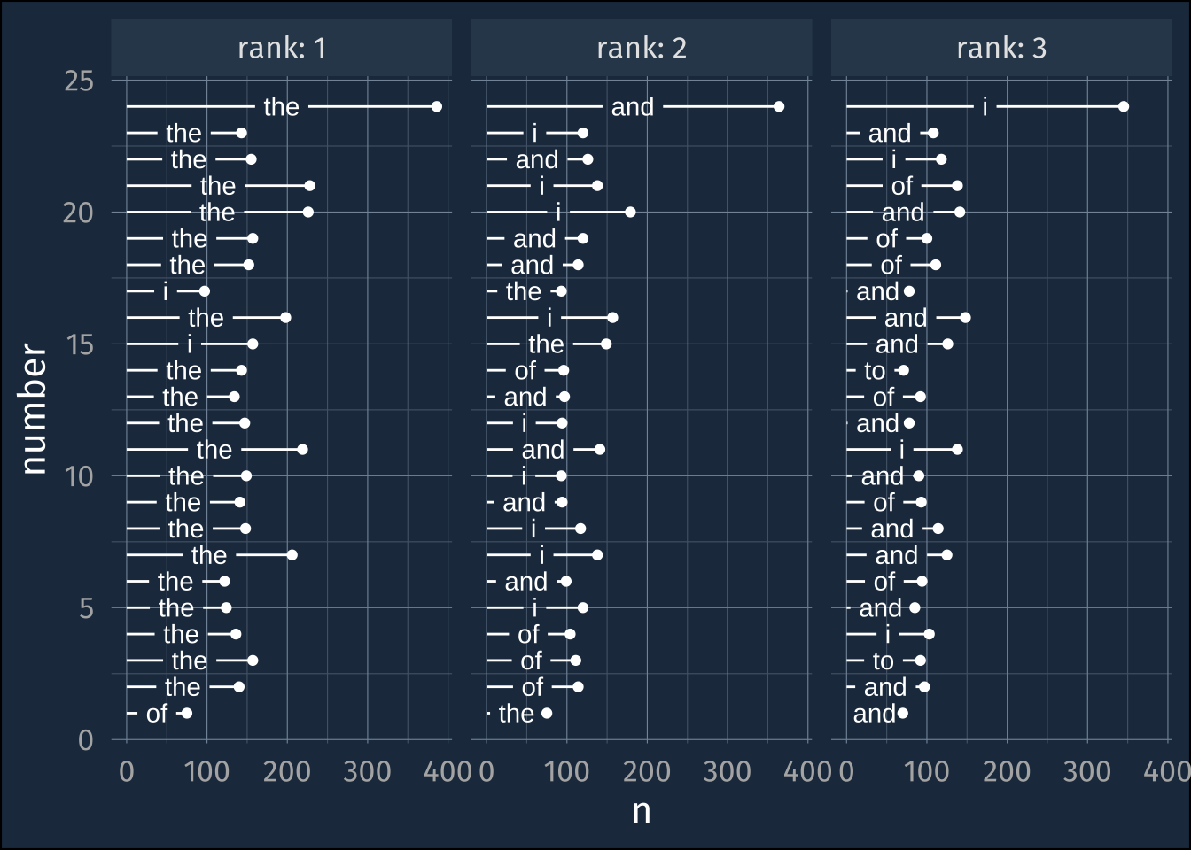

“Stopwords”

Words to just exclude from the analysis.

stop_words |> 
  count(lexicon)

# A tibble: 3 × 2
  lexicon      n
  <chr>    <int>
1 SMART      571
2 onix       404
3 snowball   174

frank_tokens |> 
  anti_join(stop_words) |> 
  count(prefix, number, word ) |> 
  group_by(prefix, number) |> 
  arrange(desc(n)) |> 
  slice(1:3) |> 
  mutate(rank = 1:3) -> 
  frequent_words2

frequent_words2 |>
  filter(prefix == "Chapter") |> 
  ggplot(aes(n, number))+
    geom_point()+
    geom_textsegment(
      aes(label = word, xend = 0, yend = number),
      color = "white"
    )+
    facet_wrap(~rank, labeller = label_both)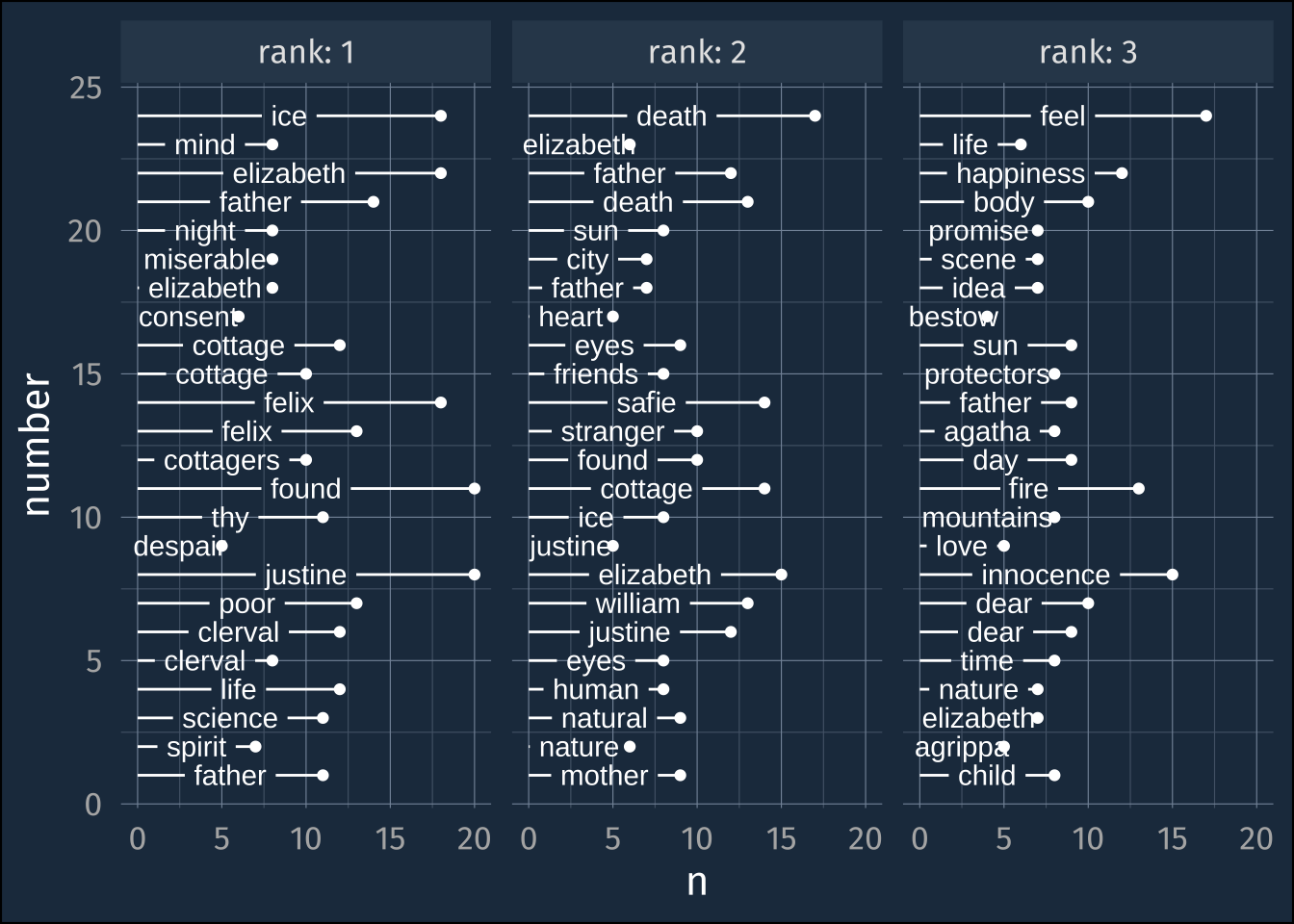

TF-IDF

TF

Term Frequency

IDF

Inverse Document Frequency

The term frequency in one document is:

\[ \frac{\text{term's frequency}}{\text{sum of all frequencies}} \]

In some sense, it becomes a normalized frequency, or a proportion of how many words were this word in the document.

Across all documents, a term shares an inverse document frequency, which is

\[ \ln\left(\frac{\text{total number of documents}}{\text{number of documents this term appeared in}}\right) \]

Illustrative example

Let’s say we have we a document with 1000 total words. Word A appeared 55 times, Word B appeared 40, times, and Word C appeared 3 times.

tribble(
  ~word, ~freq, ~total,
  "word a", 55, 1000,
  "word b", 40, 1000,
  "word c", 10, 1000
) ->
  small_example

small_example

# A tibble: 3 × 3
  word    freq total
  <chr>  <dbl> <dbl>
1 word a    55  1000
2 word b    40  1000
3 word c    10  1000

Calculating term frequency

small_example |> 
  mutate(tf = freq/total) -> 
  small_example_tf

small_example_tf |> 
  ggplot(aes(freq, tf))+
    geom_text(aes(label = word))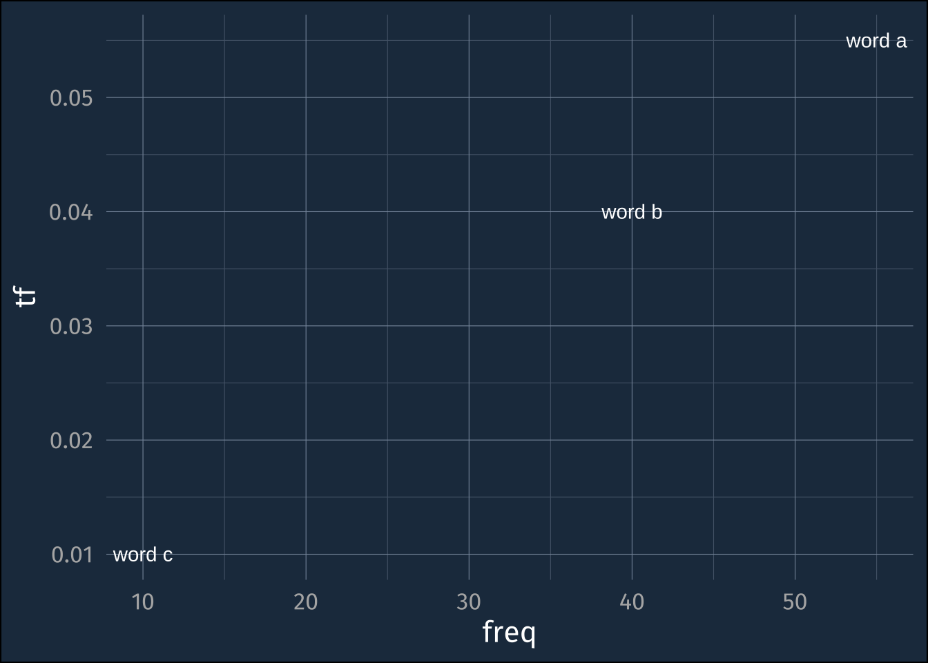

Now, let’s say we looked at whether or not each word appeared in this document and 3 other additional documents.

• Word A appeared in all 4

• Word B appeared in 2

• Word C appeared in just 1

small_example_tf |> 
  mutate(document_frequency = c(4, 2, 1),
         total_documents = 4,
         idf = log(total_documents / document_frequency)) ->
  small_example_tf_idf

small_example_tf_idf

# A tibble: 3 × 7
  word    freq total    tf document_frequency total_documents   idf
  <chr>  <dbl> <dbl> <dbl>              <dbl>           <dbl> <dbl>
1 word a    55  1000 0.055                  4               4 0    
2 word b    40  1000 0.04                   2               4 0.693
3 word c    10  1000 0.01                   1               4 1.39 

small_example_tf_idf |> 
  ggplot(aes(document_frequency, idf))+
    geom_text(aes(label = word))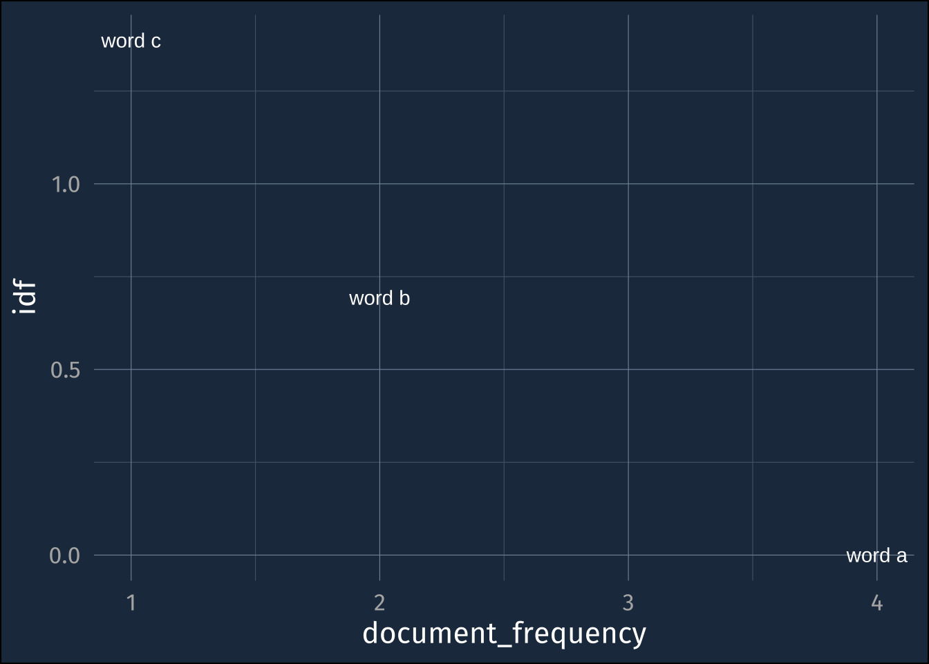

tf-idf tries to trade off between these two signals of importance by just multiplying together tf and idf

small_example_tf_idf |> 
  ggplot(aes(word, tf*idf))+
    geom_col(fill = "white")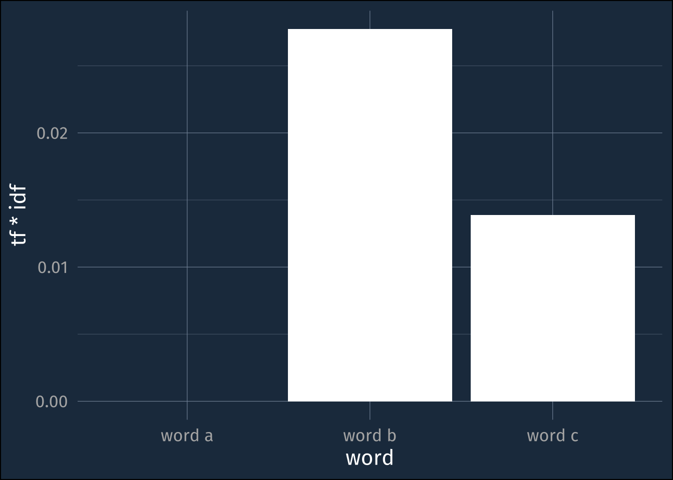

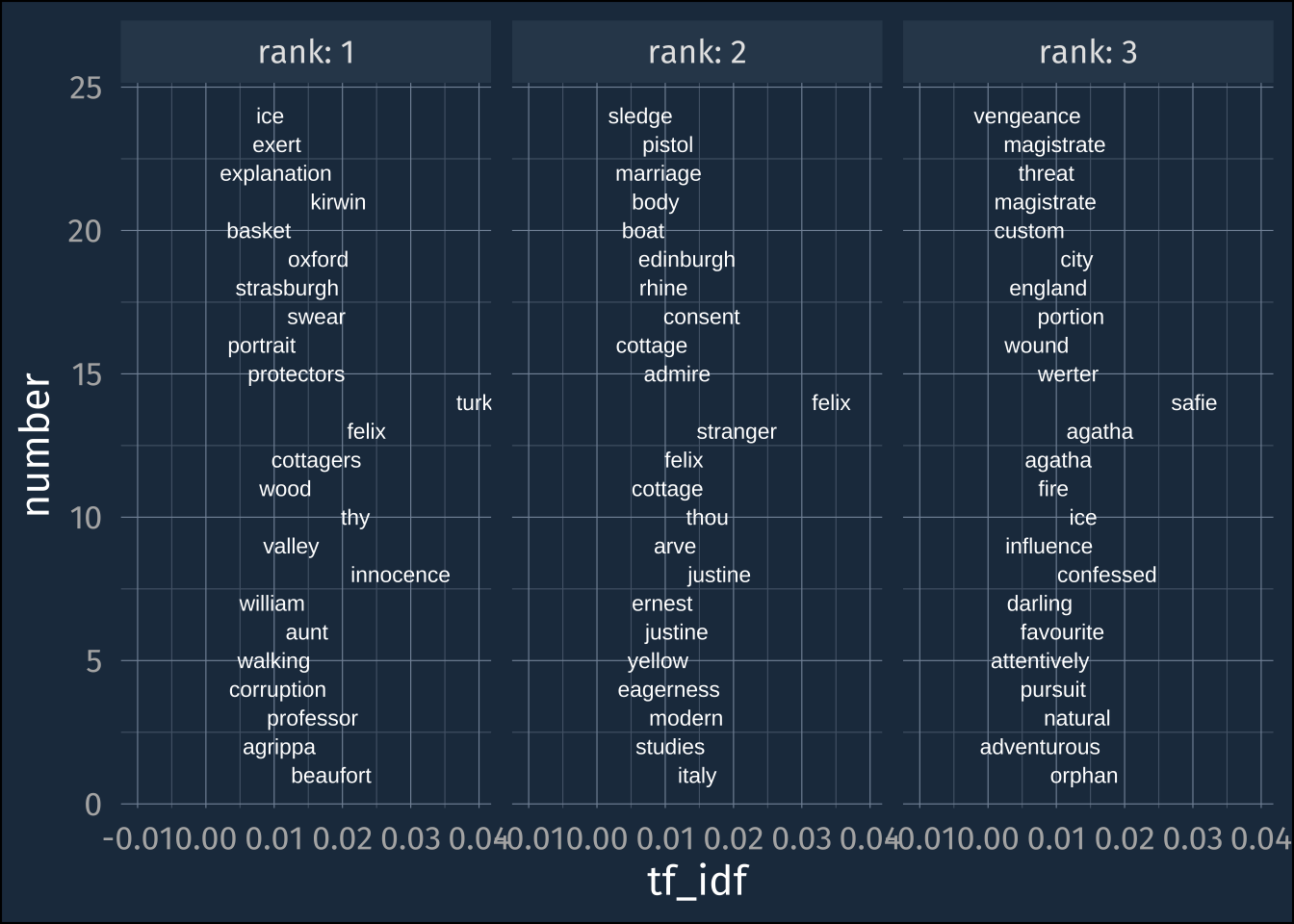
Calculating it with a real example

frank_tokens |> 
  filter(prefix == "Chapter") |> 
  count(number, word) ->
  chapter_word_counts

chapter_word_counts |> 
  anti_join(stop_words) |> 
  bind_tf_idf(word, number, n) ->
  chapter_tf_idf

chapter_tf_idf |> 
  arrange(desc(tf_idf)) |> 
  group_by(number) |> 
  slice(1:3) |> 
  mutate(rank = 1:3)->
  high_tf_idf

high_tf_idf |> 
 ggplot(aes(tf_idf, number))+
    geom_text(
      aes(label = word),
      color = "white",
      size = 3
    )+
    expand_limits(x = -0.01)+
    facet_wrap(~rank, labeller = label_both)