A&S500/Lin517 - Starting with Text

We did “strings”, but “text” is different.

library(tidyverse)

String operations are going to be things like “split a string into substrings”

String things

Here’s using directory names from the `course_notes` site as an example

library(fs)

fs::dir_ls("..") |>
  str_remove("../") ->
  notes_directory

tibble(
  notes = notes_directory
)->
  notes_df

notes_df |>
  rmarkdown::paged_table()

1: This gets a list of all files and directories in the directory above.
2: This removes the ../ component of the directory names.
3: Putting it in a tibble so we can to tibble things.

notes_df |> 
  filter(
    str_starts(notes, "2023")
  ) |> 
  separate_wider_delim(
    notes, 
    delim = "_",
    names = c("date", "name"),
    too_few = "align_start"
  ) |> 
  rmarkdown::paged_table()

Text Stuff

But text, or written language is a bit different.

sentence <- "Call me Ishmael. Some years ago—never mind how long precisely—having little or no money in my purse, and nothing particular to interest me on shore, I thought I would sail about a little and see the watery part of the world."

sentences_df <- tibble(
  sentence = sentence
)

sentences_df |> 
  rmarkdown::paged_table()

How do we split this up? Are “words” just where the spaces go?

sentences_df |> 
  separate_longer_delim(
    sentence,
    delim = " "
  ) |> 
  rmarkdown::paged_table()

What even is a word??

tribble(
  ~lexeme, ~baseform, ~contraction,
  "be", "are", "aren't",
  "be", "is", "isn't",
  "be", "was", "wasn't",
  "be", "were", "weren't",
  "do", "do", "don't",
  "do", "does", "doesn't",
  "do", "did", "didn't",
  "will", "will", "won't",
  "can", "can", "can't",
  "could", "could", "couldn't",
  "would", "would", "wouldn't"
) ->
  not_contractions

not_contractions |> 
  rmarkdown::paged_table()

If we wanted to treat the contraction as something separate from the word it’s contracted onto…¹

not_contractions |> 
  mutate(
    minus_contraction = str_remove(contraction, "n't")
  ) |> 
  filter(
    baseform != minus_contraction
  )

# A tibble: 2 × 4
  lexeme baseform contraction minus_contraction
  <chr>  <chr>    <chr>       <chr>            
1 will   will     won't       wo               
2 can    can      can't       ca

Usually text we might want to analyze is caught up in a lot of markup!

tibble(
  website = read_lines("https://www.uky.edu/", n_max = 50)
) |> 
  rmarkdown::paged_table()

Or, heaven forbid, we want to analyze text that’s in a pdf.

Getting started

Key libraries:

# Tidytext
if(!require(tidytext)){
  install.packages("tidytext")
}

# gutenbergr
if(!require(gutenbergr)){
  install.packages("gutenbergr")
}

# tidytext
if(!require(readtext)){
  install.packages("readtext")
}

# quanteda
if(!require(quanteda)){
  install.packages("quanteda")
}

# text
if(!require(text)){
  install.packages("text")
}

Tidytext and tokenizing

We’ll be following Text Mining with R.

A token is a meaningful unit of text, most often a word, that we are interested in using for further analysis, and tokenization is the process of splitting text into tokens.

sentences_df |> 
  unnest_tokens(text, sentence, token = "words")

# A tibble: 43 × 1
   text   
   <chr>  
 1 call   
 2 me     
 3 ishmael
 4 some   
 5 years  
 6 ago    
 7 never  
 8 mind   
 9 how    
10 long   
# … with 33 more rows

wuthering_heights <- gutenberg_download(768)

wuthering_heights |> 
  slice(1:10) |> 
  rmarkdown::paged_table()

We can unnest words

wuthering_heights |> 
  unnest_tokens(word, text, token = "words")  |> 
  slice(1:10) |> 
  rmarkdown::paged_table()

We can unnest sentences

wuthering_heights |> 
  summarise(
    one_big_line = str_flatten(text, collapse = " ")
  ) |> 
  unnest_tokens(sentence, one_big_line, token = "sentences") |> 
  slice(1:10) |> 
  rmarkdown::paged_table()

We can unnest ngrams

wuthering_heights |> 
  summarise(
    one_big_line = str_flatten(text, collapse = " ")
  ) |> 
  unnest_tokens(sentence, one_big_line, token = "ngrams",  n = 2) |> 
  slice(1:10) |> 
  rmarkdown::paged_table()

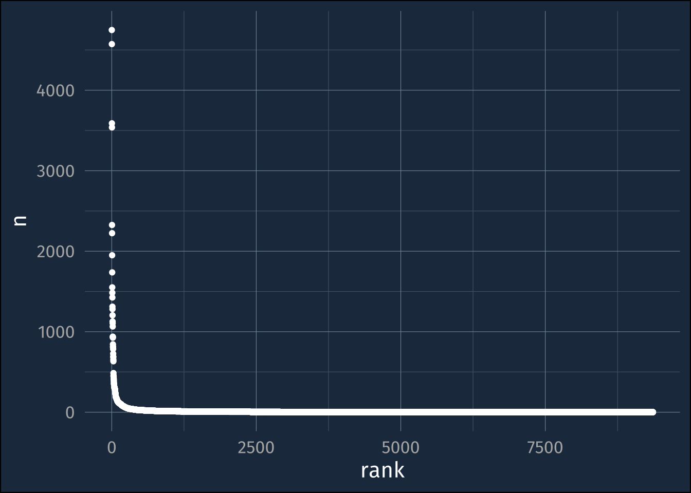
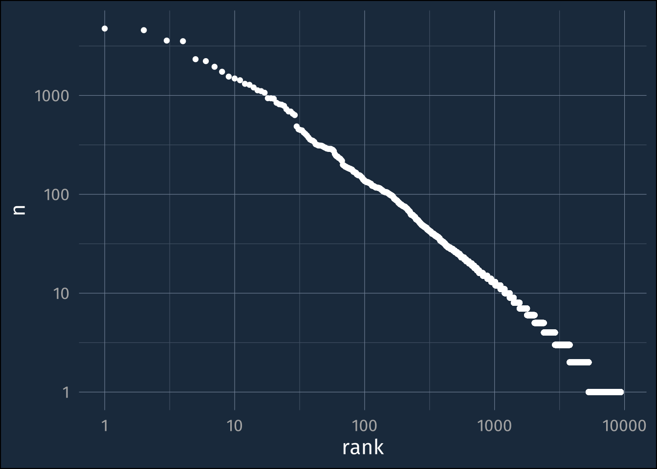
The classic power law

We can do some basics of lexicostatistics

wuthering_heights |> 
  unnest_tokens(word, text, token = "words") |>
  mutate(word = str_remove_all(word, "_")) |>
  count(word) |>
  mutate(
    rank = rank(
      desc(n),
      ties.method = "random"
    )
  ) ->
  wh_freqs

1: unnesting each token onto its own line
2: removing underscores
3: counting how often each word appeared
4: adding on word ranks (most frequent = 1, second most 2, etc)

wh_freqs |> 
  ggplot(aes(rank, n))+
    geom_point()

wh_freqs |> 
  ggplot(aes(rank, n))+
    geom_point() +
    scale_x_log10()+
    scale_y_log10()

Footnotes

We only got lucky her with “don’t”.↩︎