── Attaching packages ─────────────────────────────────────── tidyverse 1.3.2 ──
✔ tibble 3.1.8 ✔ dplyr 1.1.0
✔ tidyr 1.3.0 ✔ stringr 1.5.0
✔ readr 2.1.3 ✔ forcats 0.5.2
✔ purrr 1.0.1
── Conflicts ────────────────────────────────────────── tidyverse_conflicts() ──
✖ dplyr::filter() masks stats::filter()
✖ dplyr::lag() masks stats::lag()Census
In order to load this data, you’ll have to download it yourself from the Lexington data hub.
lex_data <- read_csv("data/Census_2020_-_Race_18_and_Over_by_Precinct.csv")Here’s what the data looks like
head(lex_data) |>
rmarkdown::paged_table()This data isn’t especially “tidy”. There is 1 row per precinct, and the column names are not descriptive. If you google the first column ID, you’ll find some tables that provide descriptive labels that look like this:
| label | id |
|---|---|
| Total: | P0030001 |
| Population of one race: | P0030002 |
| White alone | P0030003 |
| Black or African American alone | P0030004 |
| American Indian and Alaska Native alone | P0030005 |
| Asian alone | P0030006 |
| Native Hawaiian and Other Pacific Islander alone | P0030007 |
| Some Other Race alone | P0030008 |
| Two or More Races: | P0030009 |
| … | … |
A few things to note:
- We need to get these descriptive labels into the census data.
- There are data columns associated with summary values (e.g. “Total:” as well as with unsummarized data.
Step 1 requires a “data dictionary”, which you can load with the following line of code1:
source("https://jofrhwld.github.io/AandS500_2023/class_notes/2023-02-16_realmessy/data_dictionary.R")race_id |>
rmarkdown::paged_table()Some more things to note:
- Not everyone who included “Black or African American” (for example) on the census is represented in the “Black or African American Alone” data.
- The total number of people who included “Black or African American” on the census will have their data distributed across many different columns in
lex_data.
race_id |>
filter(str_detect(label, "Black or African American")) |>
rmarkdown::paged_table()There are 32 different data columns that include people who included “Black or African American” on the census.
Step 1: Pivot longer
We need to pivot lex_data long. We only want to pivot the data columns starting with "P003" long, so we’ll use starts_with() for that.
lex_data |>
pivot_longer(
starts_with("P003"),
names_to = "id",
values_to = "n"
) ->
lex_longThe dataframe lex_long now has 1 row for every P003* data column for every precinct.
Step 2: Joining
I planned ahead with the names_to="id" argument in pivot_longer() so that I could quickly join the race_id data dictionary onto it.
Joining with `by = join_by(id)`Now, we have descriptive labels on the data!
Step 3: Subdividing summary from detailed data.
One problem remaining is that there are still summary data rows in among our detailed data. The total population of each precinct is has a row, along with the detailed race identification. We’ll want to subdivide these out into different dataframes.
lex_labelled |>
filter(
str_detect(label, "Total")
) ->
lex_totals
lex_labelled |>
filter(
str_detect(label, "Population")
) ->
lex_popof
lex_labelled |>
filter(
str_detect(label, "Total", negate = T),
str_detect(label, "Population", negate = T)
) ->
lex_detailedNow, lex_detailed contains just the detailed information on what race people included in the census.
Step 4: String work
There’s a few more things we’ll want to do before we make the data as granular as possible.
- When people included just one race on the census, the label has
" alone"at the end, which we’ll want to remove to make the label align with the multiple race ids. - We’ll want to get a count of how many races people included before we break up the data.
For the first issue, we’ll use stringr::str_remove(), and for the second, we’ll use stringr::str_count() to count how many semicolons are in each label.
lex_detailed |>
mutate(
label = str_remove(label, " alone"),
n_id = str_count(label, ";") + 1,
with_id = row_number()
) ->
lex_detailed_tidyStep 5: Separating long
Now, we’ll want to separate the label column long, with a new row for each label, separating by "; "
lex_detailed_tidy |>
separate_longer_delim(label, delim = "; ") ->
lex_detailed_longSome Dataviz
Now, a thing to keep in mind is that individual people are now double counted in lex_detailed_long. For example, before we separated long, there was just 1 row for the 35 people in Gibson Park who included both “White” and “Black or African American” on the census.
lex_detailed_tidy |>
select(NAME, label, n, n_id, with_id) |>
filter(
label == "White; Black or African American",
n_id == 2,
NAME == "GIBSON PARK"
) |>
rmarkdown::paged_table()After we separated long, all 35 of these people appear in both the “White” and the “Black or African American” rows.
lex_detailed_long |>
select(NAME, label, n, n_id, with_id) |>
filter(
with_id == 511
) |>
rmarkdown::paged_table()Keeping that in mind, this is the easiest format to count up everyone who included a specific race identity in the census, whether that was “alone” or along with multiple. We can also count up how many people included multiple race identities.
lex_detailed_long |>
# Count the total number of people
# who included a race on the census
# by the number of races they included
summarise(
.by = c(label, n_id),
n = sum(n)
) |>
# Calculate the proportion of people
# who put down N race ids
# by race id
mutate(
.by = label,
prop = n/sum(n)
) |>
ggplot(aes(n_id, prop)) +
geom_col(fill = "grey90") +
ylim(0,1)+
facet_wrap(~str_wrap(label, 15)) +
theme(strip.text = element_text(size = 12))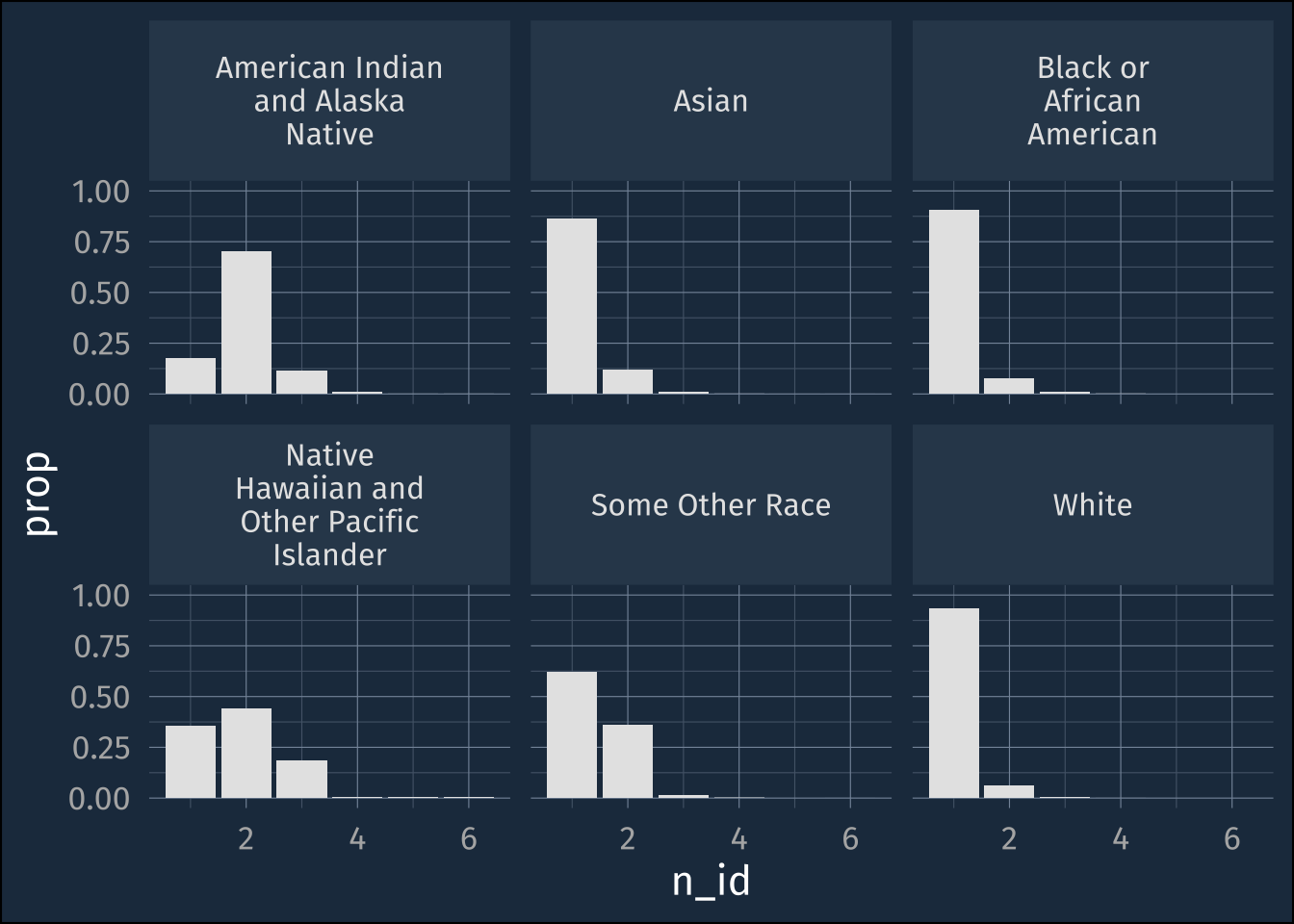
For some race ids, the most common response was just to put down just 1, but for others, like American Indian and Alaska Native, the most common response was to include 2 race ids. If we had made maps or did other analyses, and used just the data from “American Indian and Alaska Native alone”, we would have dramatically undercounted all of the people who included American Indian and Alaska Native on their census.
Footnotes
I “baked this at home” with a lot of copy-pasting from a pdf.↩︎