More working with babynames
Load up the libraries
Read in a dataframe of automatically generated pronunciations.
name_pronunciation <- read_csv("https://jofrhwld.github.io/AandS500_2023/data/name_pronunciation.csv")Recapping
We need to do some data processing to get it into a format that works well with plotting.
babynames |>
  filter(name == "Mary") |>
  ggplot(aes(x = year, y= n, color = sex)) +
    geom_line() +
    scale_color_brewer(palette = "Dark2")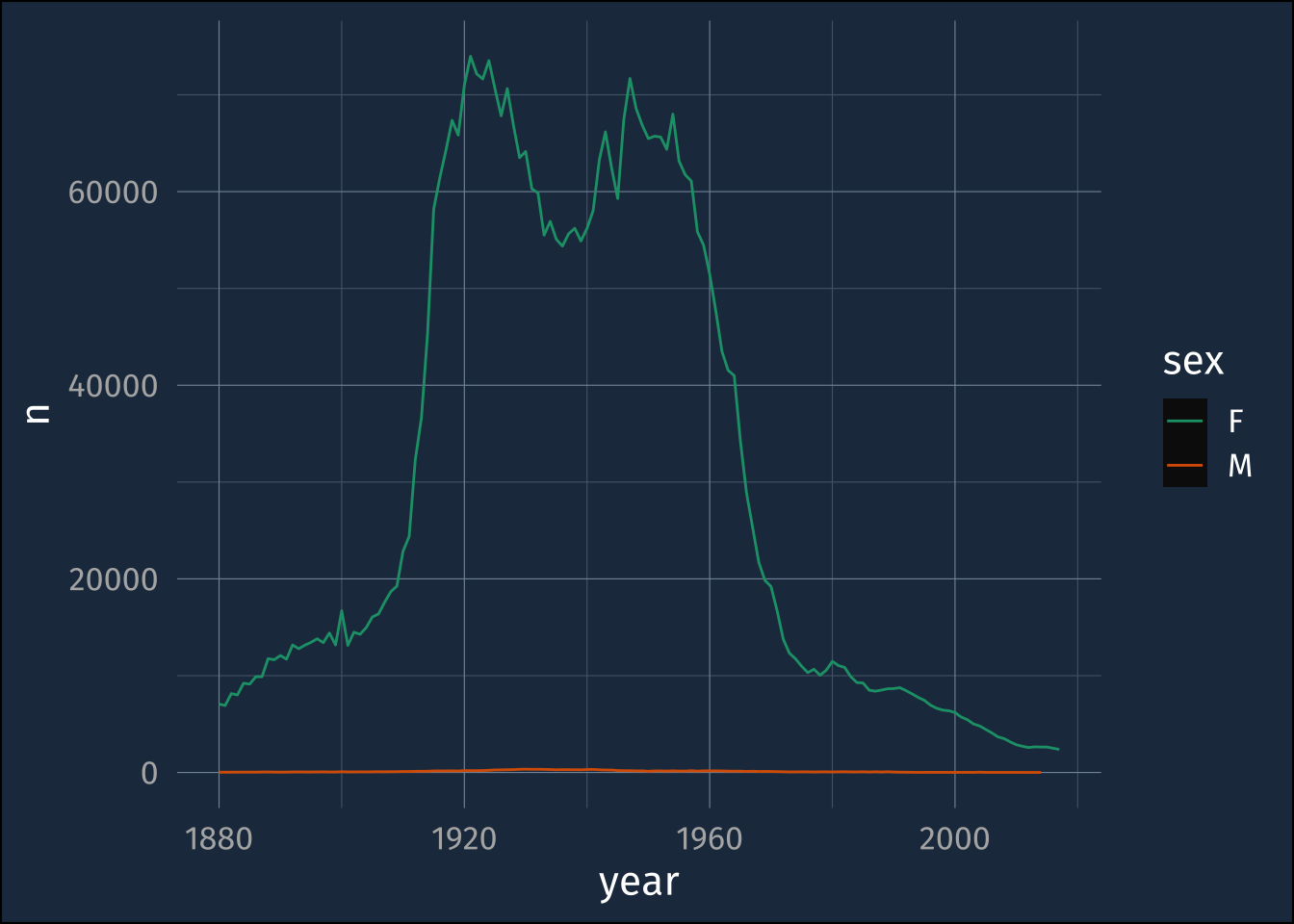
Adding new columns and summarizing
Re-coding
The function case_when() will recode data. What you give it is
<logical statement> ~ <new value>
It evaluates the logical statements in sequence.
data.frame(
name = c("Joe", "Paul", "Kate", "Rebecca", "Lil")
) |>
mutate(
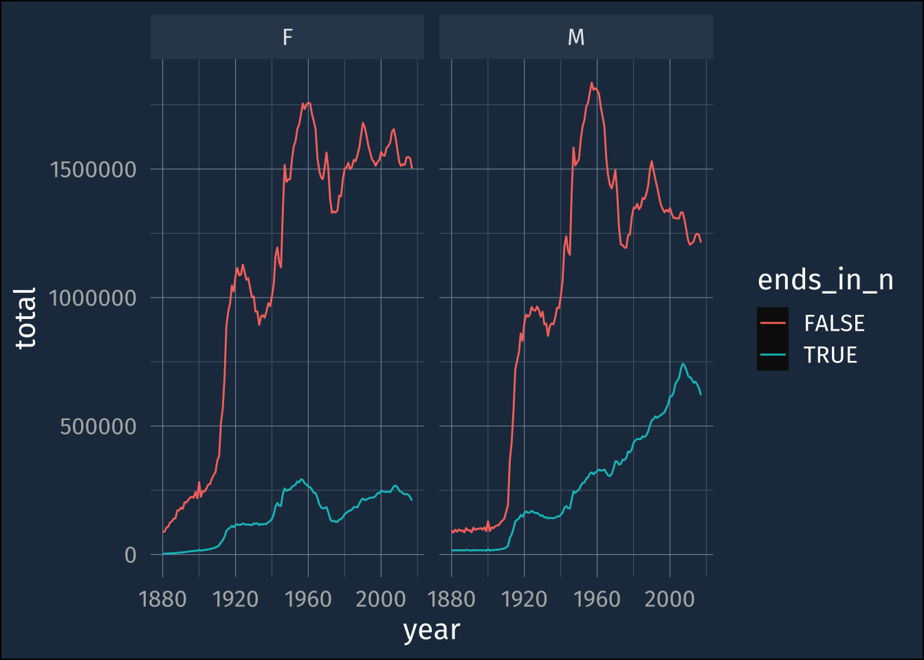
ends_in = case_when(
name == "Paul" ~ "l",
str_ends(name, "e") ~ "e",
.default = "other"
)
) name ends_in
1 Joe e
2 Paul l
3 Kate e
4 Rebecca other
5 Lil otherRecoding starwars characters’ heights into tall, medium, short.
starwars |>
  select(name, height) |>
  mutate(
    height_category = case_when(
      height >= 200 ~ "tall",
      height >= 100 ~ "medium",
      height >= 0 ~ "short",
      .default = "unrecorded"
    )
  ) |>
  arrange(desc(height)) |>
  summarise(
    .by = height_category,
    average = mean(height, na.rm = T),
    n = n()
  )
# A tibble: 4 × 3
height_category average n
<chr> <dbl> <int>
1 tall 220. 11
2 medium 176. 63
3 short 88 7
4 unrecorded NaN 6whose height isn’t there
# A tibble: 6 × 14
name height mass hair_…¹ skin_…² eye_c…³ birth…⁴ sex gender homew…⁵
<chr> <int> <dbl> <chr> <chr> <chr> <dbl> <chr> <chr> <chr>
1 Arvel Crynyd NA NA brown fair brown NA male mascu… <NA>
2 Finn NA NA black dark dark NA male mascu… <NA>
3 Rey NA NA brown light hazel NA fema… femin… <NA>
4 Poe Dameron NA NA brown light brown NA male mascu… <NA>
5 BB8 NA NA none none black NA none mascu… <NA>
6 Captain Pha… NA NA unknown unknown unknown NA <NA> <NA> <NA>
# … with 4 more variables: species <chr>, films <list>, vehicles <list>,
# starships <list>, and abbreviated variable names ¹hair_color, ²skin_color,
# ³eye_color, ⁴birth_year, ⁵homeworldJoining
Joining together datasets that have a shared “key”.
name_pronunciation <- read_csv("https://jofrhwld.github.io/AandS500_2023/data/name_pronunciation.csv")This is a dataframe with a name column shared withbabynames and pronunciation guesses.
name_pronunciation |> head()# A tibble: 6 × 2
name name_pronounce
<chr> <chr>
1 Mary M EH1 R IY0
2 Anna AE1 N AH0
3 Emma EH1 M AH0
4 Elizabeth IH0 L IH1 Z AH0 B AH0 TH
5 Minnie M IH1 N IY0
6 Margaret M AA1 R G ER0 IH0 T babynames |> head()# A tibble: 6 × 5
year sex name n prop
<dbl> <chr> <chr> <int> <dbl>
1 1880 F Mary 7065 0.0724
2 1880 F Anna 2604 0.0267
3 1880 F Emma 2003 0.0205
4 1880 F Elizabeth 1939 0.0199
5 1880 F Minnie 1746 0.0179
6 1880 F Margaret 1578 0.0162Using left_join() will return every row from the “left hand” data frame, and ever matching value from the “right hand” data frame.
# A tibble: 6 × 6
   year sex   name          n   prop name_pronounce
  <dbl> <chr> <chr>     <int>  <dbl> <chr>
1  1880 F     Mary       7065 0.0724 M EH1 R IY0
2  1880 F     Anna       2604 0.0267 AE1 N AH0
3  1880 F     Emma       2003 0.0205 EH1 M AH0
4  1880 F     Elizabeth  1939 0.0199 IH0 L IH1 Z AH0 B AH0 TH
5  1880 F     Minnie     1746 0.0179 M IH1 N IY0
6 1880 F Margaret 1578 0.0162 M AA1 R G ER0 IH0 T # A tibble: 6 × 6
year sex name n prop name_pronounce
<dbl> <chr> <chr> <int> <dbl> <chr>
1 1880 F Lee 28 0.000287 L IY1
2 1880 M Lee 361 0.00305 L IY1
3 1881 F Lee 39 0.000395 L IY1
4 1881 M Lee 342 0.00316 L IY1
5 1882 F Lee 43 0.000372 L IY1
6 1882 M Lee 427 0.00350 L IY1 Now we can filter by pronunciation and look at the most popular spellings
bn_with_pron |>
  filter(name_pronounce == "L IY1") |>
  summarise(
    .by = c(year, sex, name),
    total = sum(n)
  ) |>
  ggplot(aes(year, total, color = name))+
    geom_line()+
    facet_wrap(~sex)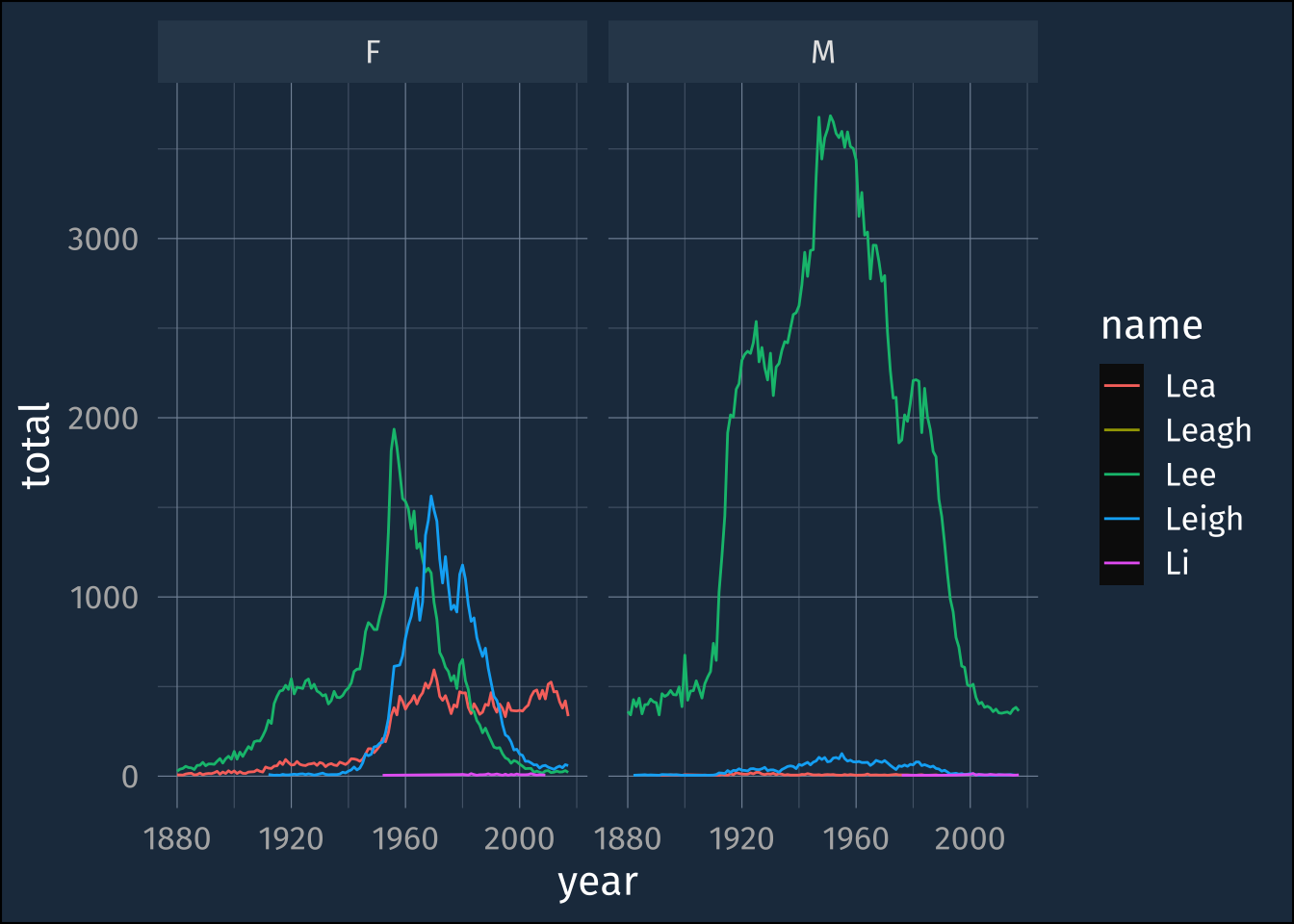
We didn’t get to this.
# name_pronunciation |>
#   select(name_pronounce) |>
#   distinct() |>
#   mutate(nsyl = str_count(name_pronounce, r"([AEIOU].\d)"))