library(tmap)
library(gifski)Loading Packages
New for today
Old news
library(tidyverse)
library(units)
library(sf)
library(terra)
library(tigris)
library(mapview)
Downloading some data
lex_councils <- read_sf("https://services1.arcgis.com/Mg7DLdfYcSWIaDnu/arcgis/rest/services/Council_District/FeatureServer/0/query?outFields=*&where=1%3D1&f=geojson")lex_bike <- read_sf("https://services1.arcgis.com/Mg7DLdfYcSWIaDnu/arcgis/rest/services/Bicycle_Network/FeatureServer/0/query?outFields=*&where=1%3D1&f=geojson")ky <- counties(state = "KY", cb = T)lex <- ky |> filter(NAME == "Fayette")Map Plots
Default plotting
lex_councils |>
  mutate(area = st_area(geometry))->
lex_councilsplot(lex_councils)Warning: plotting the first 10 out of 13 attributes; use max.plot = 13 to plot
all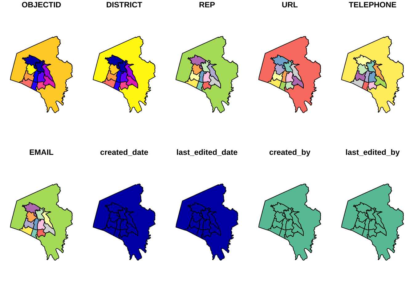
mapview
mapview(lex_councils)ggplot2
ggplot()+
  geom_sf(data = lex_councils)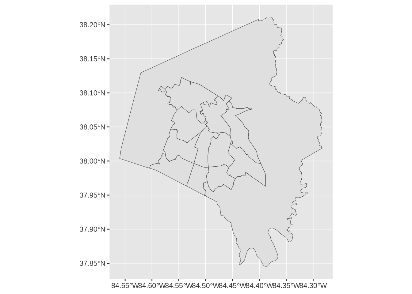
tmap
Seems to have a number of defaults set to be more pleasant for maps.
tm_shape(lex_councils)+
  tm_fill()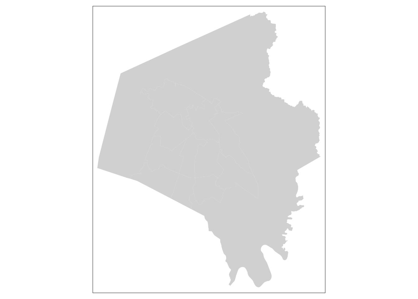
tm_shape(lex_councils)+
  tm_borders()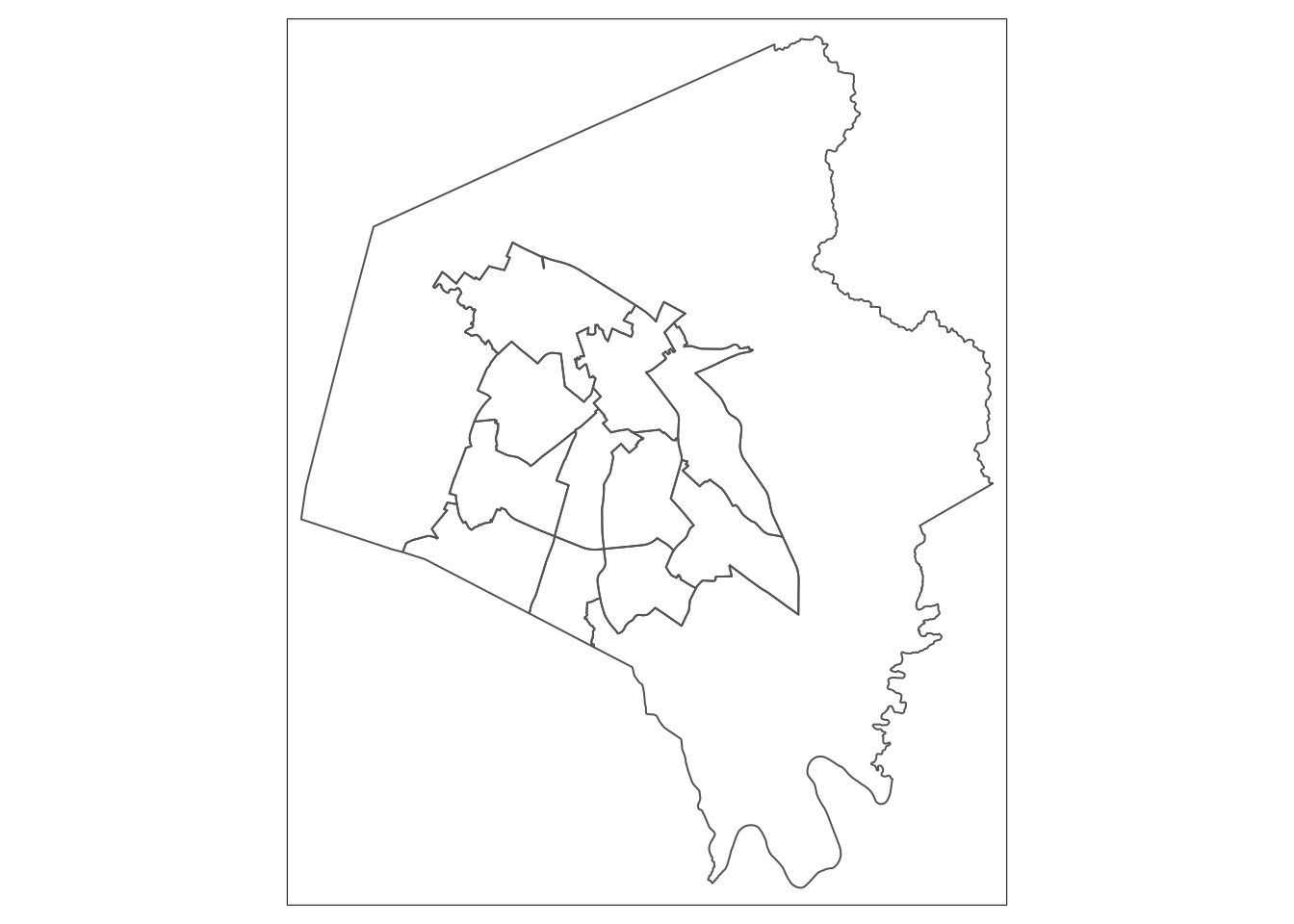
tm_shape(lex_councils)+
  tm_fill()+
  tm_borders()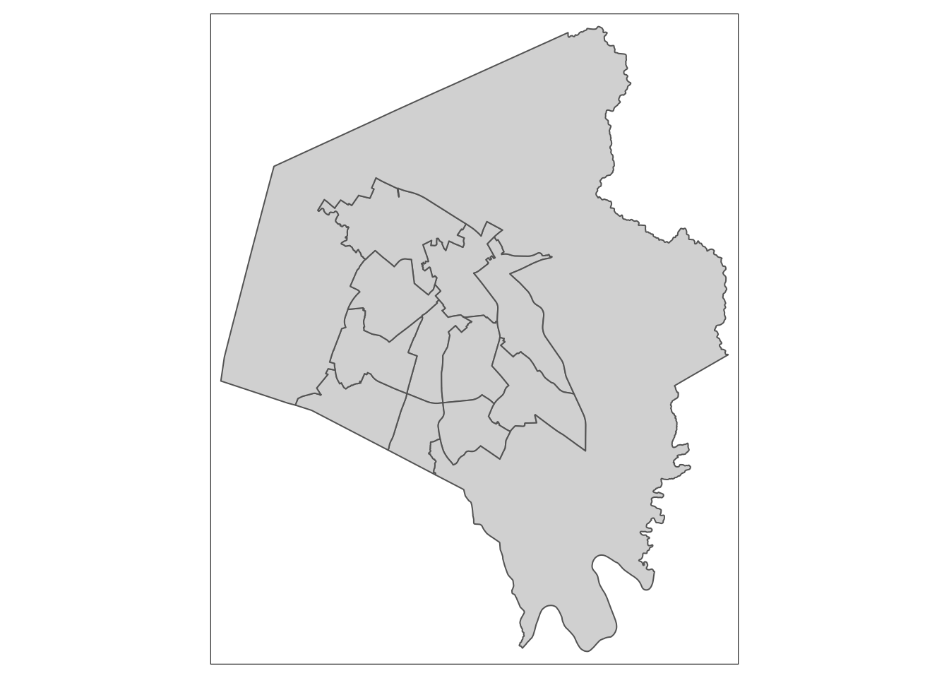
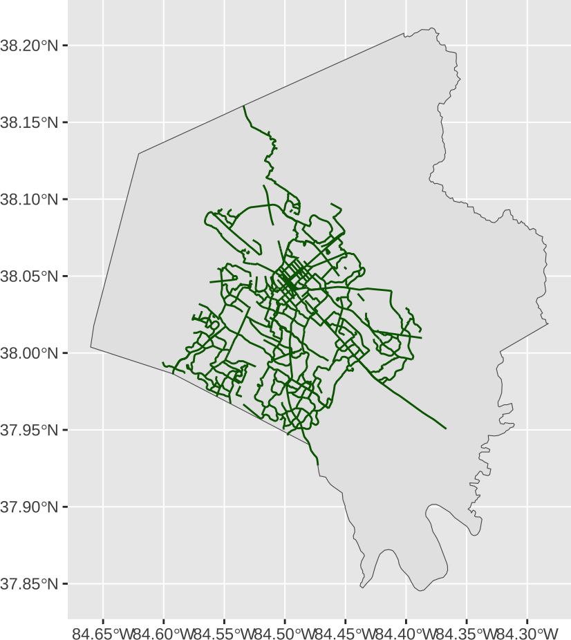
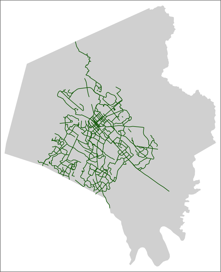
There are also some additional layers that are very map specific.
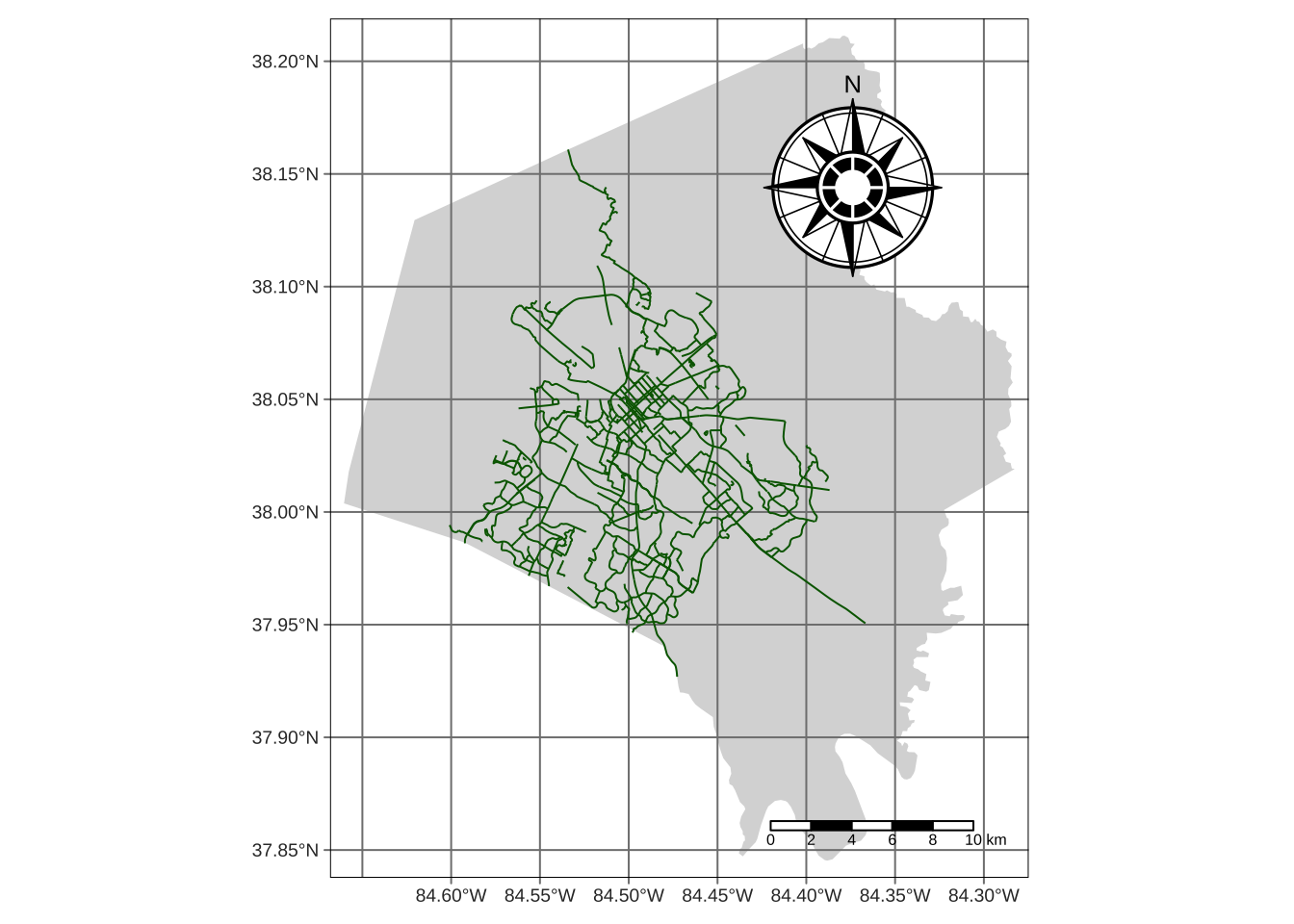
tm_shape(lex)+
tm_fill()+
tm_shape(lex_bike)+
tm_graticules()+
tm_lines(col = "darkgreen")+
tm_compass(type = "rose",
position = c(0.6, 0.7))+
tm_scale_bar()- 1
- “graticule” is the longitude and latitude lines
- 2
- There are a few different compass symbols that can be added
- 3
- Scalebar
“mapping” data, in the plotting sense
tm_shape(lex)+
  tm_fill()+
tm_shape(lex_bike)+
  tm_lines(col = "Type_Facility")+
  tm_facets(by = c("Status"), free.coords = F)+
  tm_style("col_blind")+
tm_scale_bar() 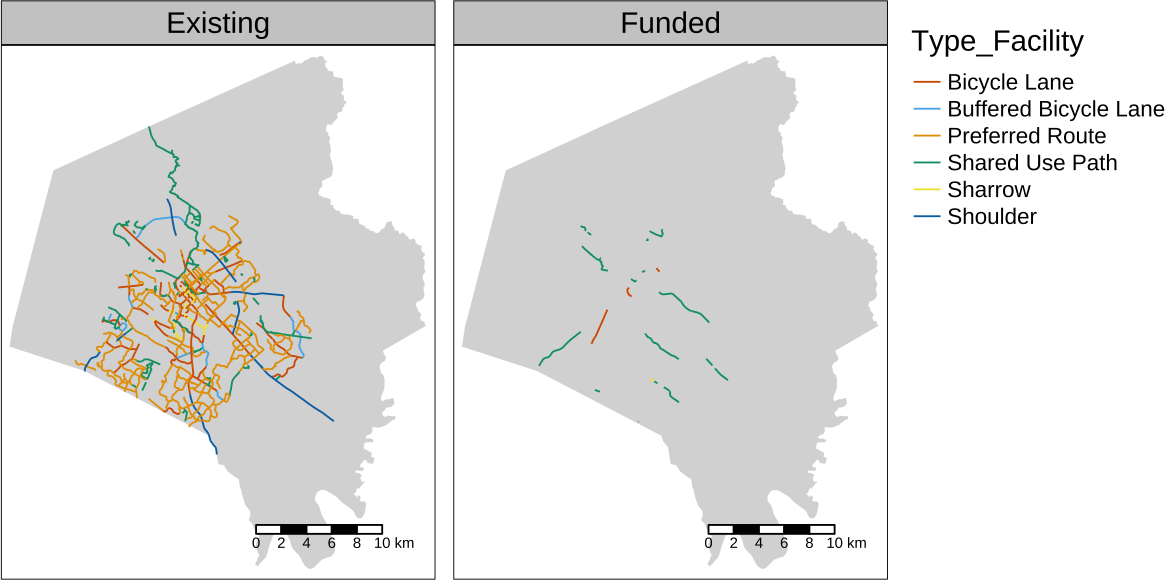
Animated Maps
tm_shape(lex) +
  tm_fill() +
tm_shape(lex_bike)+
  tm_lines()+
  tm_facets(along = "YearComplete", free.coords = F) ->
  bike_anim
This was not successful
tmap_animation(bike_anim, filename = "bike_anim.gif", delay = 25)
tmap_animation(bike_anim2, filename = "bike_anim2.gif", delay = 40)Making it work
lex_bike |>
replace_na(list(YearComplete = min(lex_bike$YearComplete, na.rm = T)))->
lex_bike
min_year <- lex_bike |> filter(YearComplete >0) |> pull(YearComplete) |> min()
max_year <- lex_bike |> filter(YearComplete >0) |> pull(YearComplete) |> max()
tibble(
anim_year = min_year:max_year
) |>
left_join(
lex_bike,
by = join_by( anim_year >= YearComplete)) |>
st_sf() ->
lex_bike_to_anim
tm_shape(lex)+
tm_fill()+
tm_shape(lex_bike_to_anim)+
tm_lines(col = "Type_Facility")+
tm_facets(along = "anim_year", free.coords = F)+
tm_layout(
title = "Lexington Bike Network",
frame = FALSE
) +
tm_style("col_blind")->
bike_anim2- 1
- I had to replace missing completion years with the earliest available completion year
- 2
- Creating a data frame of all years between the first completion year and the last
- 3
- This is the fun and tricky part
- 4
- The result was technically not a spatial data frame.
Interactive Maps
lex_pop <- read_sf("https://services1.arcgis.com/Mg7DLdfYcSWIaDnu/arcgis/rest/services/Census2020_Precinct_P3_Race_18andOver/FeatureServer/0/query?outFields=*&where=1%3D1&f=geojson")tmap_mode("view")tm_shape(lex_pop)+
tm_fill(col = "P0030001", alpha = 0.7, style = "cont")+
tm_style("col_blind")Works with Rasters too
download.file(
  "https://ky.box.com/shared/static/urm3ecx8v0zi3ojxe6rpg8j586vs0qqa.zip",
  destfile = "data/elev.zip"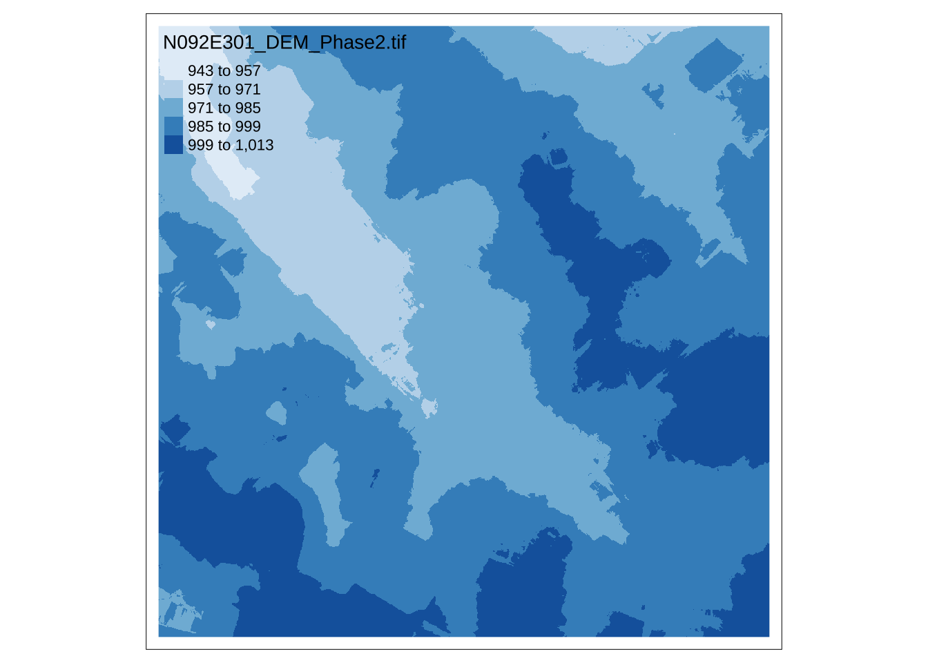
) unzip(zipfile = "data/elev.zip", exdir = "data")pot_elev <- rast("data/N092E301_DEM_Phase2.tif")tm_shape(pot_elev)+
tm_raster(alpha = 0.6)Warning: ignoring unrecognized unit: US survey foottmap_mode("plot")tm_shape(pot_elev)+
tm_raster(style = "equal")+
tm_style("col_blind")Warning: ignoring unrecognized unit: US survey foot