A&S500/Lin517 - Spatial Operations

Useful info:

Spatial Data Operations: https://r.geocompx.org/spatial-operations.html
Geometry Operations:https://r.geocompx.org/geometry-operations.html
Reprojecting geographic data: https://r.geocompx.org/reproj-geo-data.html

The Goal:

Create a “voronoi tesselation” map, dividing up the US into states where every point inside the state is closer to its own capital than any other capital.

library(tidyverse)
library(sf)
library(maps)
library(units)
library(tigris)
library(mapview)

Getting US State data

tigris::states() downloads the state border data

us_state <- states(cb = T, resolution = "5m")

head(us_state)

Simple feature collection with 6 features and 9 fields
Geometry type: MULTIPOLYGON
Dimension:     XY
Bounding box:  xmin: -94.61792 ymin: 17.87831 xmax: -65.22157 ymax: 41.97752
Geodetic CRS:  NAD83
  STATEFP  STATENS    AFFGEOID GEOID STUSPS           NAME LSAD        ALAND
1      72 01779808 0400000US72    72     PR    Puerto Rico   00   8869135605
2      22 01629543 0400000US22    22     LA      Louisiana   00 111915258185
3      24 01714934 0400000US24    24     MD       Maryland   00  25151992308
4      39 01085497 0400000US39    39     OH           Ohio   00 105823653399
5      05 00068085 0400000US05    05     AR       Arkansas   00 134660767709
6      37 01027616 0400000US37    37     NC North Carolina   00 125933327733
       AWATER                       geometry
1  4922143005 MULTIPOLYGON (((-65.3357 18...
2 23736382213 MULTIPOLYGON (((-88.88145 3...
3  6979074857 MULTIPOLYGON (((-76.04862 3...
4 10274702852 MULTIPOLYGON (((-82.73571 4...
5  3121950081 MULTIPOLYGON (((-94.61792 3...
6 13456093195 MULTIPOLYGON (((-75.72681 3...

maps::us.cities has geographic data for US cities.

head(us.cities)

        name country.etc    pop   lat    long capital
1 Abilene TX          TX 113888 32.45  -99.74       0
2   Akron OH          OH 206634 41.08  -81.52       0
3 Alameda CA          CA  70069 37.77 -122.26       0
4  Albany GA          GA  75510 31.58  -84.18       0
5  Albany NY          NY  93576 42.67  -73.80       2
6  Albany OR          OR  45535 44.62 -123.09       0

Just grabbing the data from US capitals from us.cities.

us_capitals <- us.cities |>
  filter(capital == 2)

head(us_capitals)

            name country.etc    pop   lat   long capital
1      Albany NY          NY  93576 42.67 -73.80       2
2   Annapolis MD          MD  36300 38.98 -76.49       2
3     Atlanta GA          GA 424096 33.76 -84.42       2
4     Augusta ME          ME  18626 44.32 -69.77       2
5      Austin TX          TX 683404 30.31 -97.75       2
6 Baton Rouge LA          LA 222217 30.45 -91.13       2

Making geometries

The data in us_capitals has longitude and latitude columns, not the kind of sf geometries we need to work with.

us_capitals |> 
  slice(1)

       name country.etc   pop   lat  long capital
1 Albany NY          NY 93576 42.67 -73.8       2

We can make a single sf point object like this:

st_point(c(-73.8, 42.67))

Our process for doing this is

- Use dplyr::rowwise() to tell R we’re going to do the next steps row-by-row

- Create a column simple feature points

- convert the resulting dataframe into an sf-dataframe.

us_capitals |> 
  # operate rowwise
  rowwise() |>  
  # greate the point geometries
  mutate(geometry = list(st_point(c(long, lat)))) |>
  # convert to the special sf dataframe
  st_as_sf() ->
  capitals_sf

head(capitals_sf)

Simple feature collection with 6 features and 6 fields
Geometry type: POINT
Dimension:     XY
Bounding box:  xmin: -97.75 ymin: 30.31 xmax: -69.77 ymax: 44.32
CRS:           NA
# A tibble: 6 × 7
# Rowwise: 
  name           country.…¹    pop   lat  long capital       geometry
  <chr>          <chr>       <int> <dbl> <dbl>   <int>        <POINT>
1 Albany NY      NY          93576  42.7 -73.8       2  (-73.8 42.67)
2 Annapolis MD   MD          36300  39.0 -76.5       2 (-76.49 38.98)
3 Atlanta GA     GA         424096  33.8 -84.4       2 (-84.42 33.76)
4 Augusta ME     ME          18626  44.3 -69.8       2 (-69.77 44.32)
5 Austin TX      TX         683404  30.3 -97.8       2 (-97.75 30.31)
6 Baton Rouge LA LA         222217  30.4 -91.1       2 (-91.13 30.45)
# … with abbreviated variable name ¹country.etc

capitals_sf |> 
  ggplot()+
    geom_sf()

Setting the Coordinate Reference System

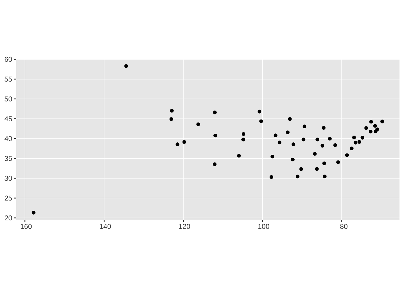
While we’ve got geographic points in the data, our mapping tools won’t know where they are without a “Coordinate Reference System.” mapview() just puts the points in a grey void without a basemap.

mapview(capitals_sf)

Coordinate Reference Systems

The world is a potato

Geoid based on the European Space Agency

“Default” CRS?

According to the Geocomputation in R book (https://r.geocompx.org/reproj-geo-data.html#which-crs), the EPSG code for the most widely used CRS is 4326.

st_crs(capitals_sf) <- 4326

After setting the CRS, mapview() will plot our points in the with a basemap.

mapview(capitals_sf)

Changing the coordinate reference system.

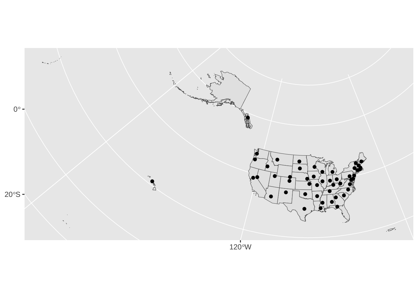
Once an sf data frame has a CRS, we can then transform it to have a different CRS (e.g. one that has a different projection, or different origin point).

us_state |>
  #using the albers conic projection
  st_transform(5070)->
  us_conus

capitals_sf |>
  st_transform(5070)->
  capitals_conus

ggplot()+
  geom_sf(data = us_conus) +
  geom_sf(data = capitals_conus)

Making the Tiles

The math behind the voronoi tesselation requires looking at all of the points at the same time, meaning we need to combine each individual point into a multipoint object.

capitals_conus |> 
  st_union()

Geometry set for 1 feature 
Geometry type: MULTIPOINT
Dimension:     XY
Bounding box:  xmin: -6121398 ymin: 805334.8 xmax: 2059946 ymax: 4368541
Projected CRS: NAD83 / Conus Albers

With this multipoint object, we can then do the voronoi tessellation

capitals_conus |> 
  st_union() |> 
  st_voronoi()

Geometry set for 1 feature 
Geometry type: GEOMETRYCOLLECTION
Dimension:     XY
Bounding box:  xmin: -14302740 ymin: -7376009 xmax: 10241290 ymax: 12549880
Projected CRS: NAD83 / Conus Albers

The outcome is a “geometry collection”, which we’ll want to convert back to a spatial column

capitals_conus |> 
  st_union() |> 
  st_voronoi() |> 
  st_collection_extract()

Geometry set for 50 features 
Geometry type: POLYGON
Dimension:     XY
Bounding box:  xmin: -14302740 ymin: -7376009 xmax: 10241290 ymax: 12549880
Projected CRS: NAD83 / Conus Albers
First 5 geometries: