Starting with Maps

Author

Josef Fruehwald

Published

February 28, 2023

── Attaching packages ─────────────────────────────────────── tidyverse 1.3.2 ──
✔ tibble  3.1.8     ✔ dplyr   1.1.0
✔ tidyr   1.3.0     ✔ stringr 1.5.0
✔ readr   2.1.3     ✔ forcats 0.5.2
✔ purrr   1.0.1     
── Conflicts ────────────────────────────────────────── tidyverse_conflicts() ──
✖ dplyr::filter() masks stats::filter()
✖ dplyr::lag()    masks stats::lag()
To enable caching of data, set `options(tigris_use_cache = TRUE)`
in your R script or .Rprofile.
Linking to GEOS 3.11.0, GDAL 3.5.3, PROJ 9.1.0; sf_use_s2() is TRUE
To access larger datasets in this package, install the spDataLarge
package with: `install.packages('spDataLarge',
repos='https://nowosad.github.io/drat/', type='source')`

sf - Simple Features

sf seems to be the most tightly integrated package into the tidyverse workflow we’ve been using.

This is basically a dataframe like any other, except for the $geom column.

## from the spData package
head(world)
Simple feature collection with 6 features and 10 fields
Geometry type: MULTIPOLYGON
Dimension:     XY
Bounding box:  xmin: -180 ymin: -18.28799 xmax: 180 ymax: 83.23324
Geodetic CRS:  WGS 84
# A tibble: 6 × 11
  iso_a2 name_long conti…¹ regio…² subre…³ type  area_…⁴     pop lifeExp gdpPe…⁵
  <chr>  <chr>     <chr>   <chr>   <chr>   <chr>   <dbl>   <dbl>   <dbl>   <dbl>
1 FJ     Fiji      Oceania Oceania Melane… Sove…  1.93e4  8.86e5    70.0   8222.
2 TZ     Tanzania  Africa  Africa  Easter… Sove…  9.33e5  5.22e7    64.2   2402.
3 EH     Western … Africa  Africa  Northe… Inde…  9.63e4 NA         NA       NA 
4 CA     Canada    North … Americ… Northe… Sove…  1.00e7  3.55e7    82.0  43079.
5 US     United S… North … Americ… Northe… Coun…  9.51e6  3.19e8    78.8  51922.
6 KZ     Kazakhst… Asia    Asia    Centra… Sove…  2.73e6  1.73e7    71.6  23587.
# … with 1 more variable: geom <MULTIPOLYGON [°]>, and abbreviated variable
#   names ¹​continent, ²​region_un, ³​subregion, ⁴​area_km2, ⁵​gdpPercap
world$geom[[2]]
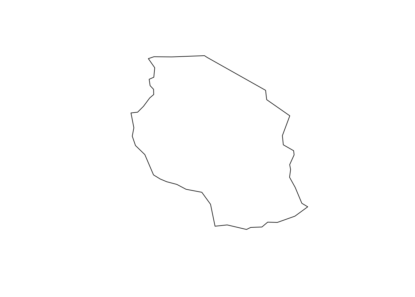
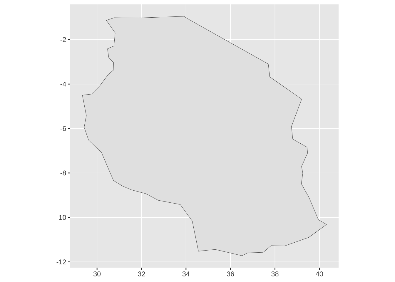
MULTIPOLYGON (((33.90371 -0.95, 31.86617 -1.02736, 30.76986 -1.01455, 30.4191 -1.134659, 30.81613 -1.698914, 30.75831 -2.28725, 30.46967 -2.41383, 30.46967 -2.413855, 30.52766 -2.80762, 30.74301 -3.03431, 30.75224 -3.35931, 30.50554 -3.56858, 30.11632 -4.09012, 29.75351 -4.452389, 29.34 -4.499983, 29.51999 -5.419979, 29.41999 -5.939999, 29.62003 -6.520015, 30.2 -7.079981, 30.74002 -8.340007, 30.74001 -8.340006, 31.15775 -8.594579, 31.55635 -8.762049, 32.19186 -8.930359, 32.75938 -9.230599, 33.73972 -9.41715, 33.94084 -9.693674, 34.28 -10.16, 34.55999 -11.52002, 35.3124 -11.43915, 36.51408 -11.72094, 36.77515 -11.59454, 37.47129 -11.56876, 37.82764 -11.26879, 38.42756 -11.2852, 39.521 -10.89688, 40.31659 -10.3171, 40.31659 -10.3171, 39.9496 -10.0984, 39.53574 -9.11237, 39.18652 -8.48551, 39.25203 -8.00781, 39.19469 -7.7039, 39.47 -7.1, 39.44 -6.84, 38.79977 -6.47566, 38.74054 -5.90895, 39.20222 -4.67677, 37.7669 -3.67712, 37.69869 -3.09699, 34.07262 -1.05982, 33.90371 -0.95)))
plot(world$geom[[2]])

ggplot(world$geom[[2]])+
    geom_sf()

world |> 
  ggplot()+
    geom_sf()

world |> 
  filter(name_long == "Brazil") -> 
  Brazil

mapview(Brazil)

Doing tidyverse things

world |> 
  group_by(subregion) |> 
  summarise(
    pop = sum(pop, na.rm = T)
  ) |> 
  ggplot()+
    geom_sf(aes(fill = log10(pop)))+
    scale_fill_batlow()

Repeating some earlier work

lex_data <- read_sf("https://services1.arcgis.com/Mg7DLdfYcSWIaDnu/arcgis/rest/services/Census2020_Precinct_P3_Race_18andOver/FeatureServer/0/query?where=1%3D1&objectIds=&time=&geometry=&geometryType=esriGeometryEnvelope&inSR=&spatialRel=esriSpatialRelIntersects&resultType=none&distance=0.0&units=esriSRUnit_Meter&relationParam=&returnGeodetic=false&outFields=*&returnGeometry=true&returnCentroid=false&featureEncoding=esriDefault&multipatchOption=xyFootprint&maxAllowableOffset=&geometryPrecision=&outSR=&defaultSR=&datumTransformation=&applyVCSProjection=false&returnIdsOnly=false&returnUniqueIdsOnly=false&returnCountOnly=false&returnExtentOnly=false&returnQueryGeometry=false&returnDistinctValues=false&cacheHint=false&orderByFields=&groupByFieldsForStatistics=&outStatistics=&having=&resultOffset=&resultRecordCount=&returnZ=false&returnM=false&returnExceededLimitFeatures=true&quantizationParameters=&sqlFormat=none&f=pgeojson&token=")
lex_data
Simple feature collection with 286 features and 76 fields
Geometry type: POLYGON
Dimension:     XY
Bounding box:  xmin: -84.66013 ymin: 37.84527 xmax: -84.28263 ymax: 38.21146
Geodetic CRS:  WGS 84
# A tibble: 286 × 77
   OBJECTID CODE  NAME   P0030…¹ P0030…² P0030…³ P0030…⁴ P0030…⁵ P0030…⁶ P0030…⁷
      <int> <chr> <chr>    <int>   <int>   <int>   <int>   <int>   <int>   <int>
 1        1 A101  ALEXA…     632     574     444      68      11      10       0
 2        2 A102  BARKER     800     754     570      86       0      66       2
 3        3 A103  BEAUM…     721     680     602      51       5       2       0
 4        4 A104  BELL …     722     645     502      11       6       8       0
 5        5 A106  CARDI…     908     787     391     166      10       4       0
 6        6 A109  DOUGL…    1356    1284     297     876       9       8       2
 7        7 A111  FAIRL…    1303    1220     774     333       8       9       1
 8        8 A113  GARDE…    1134    1062     847     135       6      21       3
 9        9 A114  GIBSO…    1394    1292     897     171       9     128       8
10       10 A115  GREEN…    1313    1261     122     935       3       2       1
# … with 276 more rows, 67 more variables: P0030008 <int>, P0030009 <int>,
#   P0030010 <int>, P0030011 <int>, P0030012 <int>, P0030013 <int>,
#   P0030014 <int>, P0030015 <int>, P0030016 <int>, P0030017 <int>,
#   P0030018 <int>, P0030019 <int>, P0030020 <int>, P0030021 <int>,
#   P0030022 <int>, P0030023 <int>, P0030024 <int>, P0030025 <int>,
#   P0030026 <int>, P0030027 <int>, P0030028 <int>, P0030029 <int>,
#   P0030030 <int>, P0030031 <int>, P0030032 <int>, P0030033 <int>, …
lex_data |> 
  select(CODE, NAME, P0030001) |> 
  rename(
    code = CODE,
    name = NAME,
    total = P0030001
  ) -> 
  lex_focus
lex_focus
Simple feature collection with 286 features and 3 fields
Geometry type: POLYGON
Dimension:     XY
Bounding box:  xmin: -84.66013 ymin: 37.84527 xmax: -84.28263 ymax: 38.21146
Geodetic CRS:  WGS 84
# A tibble: 286 × 4
   code  name               total                                       geometry
   <chr> <chr>              <int>                                  <POLYGON [°]>
 1 A101  ALEXANDRIA           632 ((-84.55478 38.02311, -84.55486 38.02305, -84…
 2 A102  BARKER               800 ((-84.52218 38.07133, -84.52394 38.06802, -84…
 3 A103  BEAUMONT             721 ((-84.5578 38.02535, -84.55787 38.02529, -84.…
 4 A104  BELL SCHOOL HOUSE    722 ((-84.52944 38.12363, -84.52914 38.12164, -84…
 5 A106  CARDINAL VALLEY      908 ((-84.54363 38.05596, -84.54381 38.05549, -84…
 6 A109  DOUGLAS-WASHINGTON  1356 ((-84.50501 38.07043, -84.5048 38.07013, -84.…
 7 A111  FAIRLAWN            1303 ((-84.47435 38.06233, -84.47498 38.06189, -84…
 8 A113  GARDEN SPRINGS      1134 ((-84.54326 38.02701, -84.54094 38.02459, -84…
 9 A114  GIBSON PARK         1394 ((-84.52361 38.04085, -84.52349 38.0407, -84.…
10 A115  GREEN ACRES         1313 ((-84.4815 38.08266, -84.48005 38.08213, -84.…
# … with 276 more rows
mapview(lex_focus, zcol = "total")

Getting data from census via tigris

MI_default <- counties(state = "MI")
Retrieving data for the year 2021
MI_cb <- counties(state = "MI", cb = T)
Retrieving data for the year 2021
MI_default |> 
  ggplot()+
    geom_sf() +
    labs(title = "default")-> mi_default_plot

MI_cb |> 
  ggplot()+
    geom_sf() +
    labs(title = "cb")-> mi_cb_plot

mi_default_plot + mi_cb_plot

ggplot()+
  geom_sf(data = MI_default, fill = "darkblue")+
  geom_sf(data = MI_cb)

lex_water <- area_water(state = "KY", county = "Fayette")
Retrieving data for the year 2021
ggplot()+
  geom_sf(data = lex_data, fill = "grey20", color = "grey20") +
  geom_sf(data = lex_water, fill = "blue", color = "blue")

Adding a buffer around the bodies of water:

ggplot()+
  geom_sf(data = lex_data, fill = "grey20", color = "grey20") +
  geom_sf(data = st_buffer(lex_water, dist = 500), fill = "lightblue", color = "lightblue")+
  geom_sf(data = lex_water, fill = "blue", color = "blue")