── Attaching packages ─────────────────────────────────────── tidyverse 1.3.2 ──
✔ tibble  3.1.8     ✔ dplyr   1.1.0
✔ tidyr   1.3.0     ✔ stringr 1.5.0
✔ readr   2.1.3     ✔ forcats 0.5.2
✔ purrr   1.0.1
── Conflicts ────────────────────────────────────────── tidyverse_conflicts() ──
✖ dplyr::filter() masks stats::filter()
✖ dplyr::lag()    masks stats::lag()
What is “tidy data”
The actual paper on the topic is worth reading: Wickham (2014). There are three rules to tidy data:
- Every column is one, and only one, variable.
- Every row is one, and only one, observation.
- Every cell is a single value.
Pivoting
install.packages("nasapower")Here is an “untidy” data set. There are multiple observations per row.
lex_temp |>
  rmarkdown::paged_table()
To tidy this data up, we need to “pivot” it longer. Simply saying pivot_longer() and telling it which columns we want to turn long-wise (JAN through DEC) will do the trick.
lex_temp |>
  pivot_longer(
    cols = JAN:DEC
  ) |>
  rmarkdown::paged_table()
Before, there was 1 row per year, and 1 column per month. Now there are 12 rows per year, with the 12 months’ column names moved into a column called name and the values in a column called value.
We can tell pivot_wider() what to call the new columns by passing it arguments to names_to= and values_to=
lex_temp |>
  pivot_longer(
    cols = JAN:DEC,
    names_to = "month",
    values_to = "temp"
  ) ->
  lex_temp_long

lex_temp_long |>
  rmarkdown::paged_table()
If we try turning this into a plot or heat map right away, it won’t go quite according to plan.
lex_temp_long |>
  ggplot(aes(month, YEAR, fill = temp))+
    geom_raster()+
    scale_fill_viridis_c(option = "magma")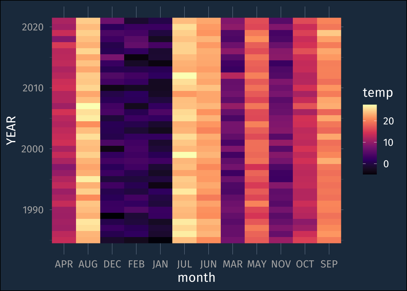
By default, it’s plotting the months in alphabetical order.
lex_temp_long |>
  mutate(month = str_to_lower(month)) |>
  ggplot(aes(month, YEAR, fill = temp))+
    geom_raster() +
    scale_fill_viridis_c(option = "magma") +
    scale_x_discrete(limits = str_to_lower(month.abb))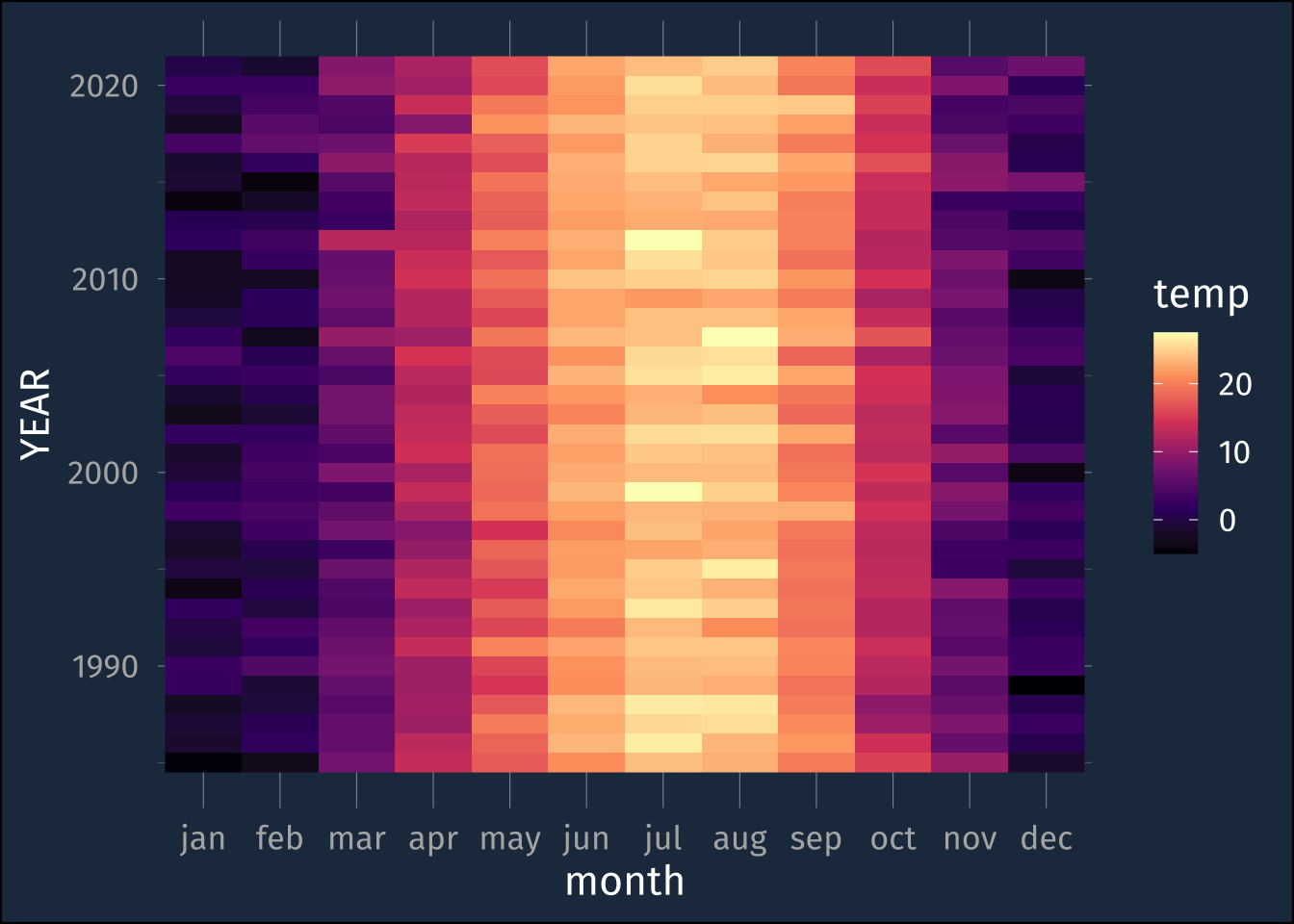
lex_temp_long |>
  mutate(month = str_to_lower(month)) |>
  ggplot(aes(YEAR, month, fill = temp))+
    geom_raster() +
    scale_fill_viridis_c(option = "magma") +
    scale_y_discrete(limits = rev(str_to_lower(month.abb)))+
    coord_fixed()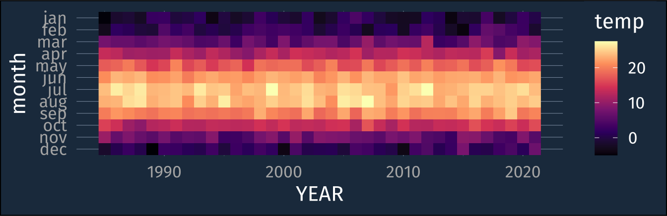
Separating
When there’s more than one value in a cell, we need to separate_ them. Let’s say three people described cities, and we recorded them in this dataframe.
tribble(
  ~person, ~city, ~description,
  "joe", "Philadelphia, PA", "Gritty, weird",
  "skylar", "Columbus, OH", "Cheap, easy, comfortable",
  "robin", "Nashville, TN", "musical"
) -> cities
cities
# A tibble: 3 × 3
person city description
<chr> <chr> <chr>
1 joe Philadelphia, PA Gritty, weird
2 skylar Columbus, OH Cheap, easy, comfortable
3 robin Nashville, TN musical The column city contains two values, the city and the state, and the column description contains between 1 and 3 values, depending on each person.
To separate the city column into a separate city and state, we need to use separate_wider_delim().
cities |>
  separate_wider_delim(
    cols = city,
    delim = ", ",
    names = c("city", "state")
  )
# A tibble: 3 × 4
person city state description
<chr> <chr> <chr> <chr>
1 joe Philadelphia PA Gritty, weird
2 skylar Columbus OH Cheap, easy, comfortable
3 robin Nashville TN musical We’ll want to separate the description column into different rows, which we can do with separate_longer_delim().
cities |>
  separate_wider_delim(
    cols = city,
    delim = ", ",
    names = c("city", "state")
  ) |>
  separate_longer_delim(
    cols = description,
    delim = ", "
  )
# A tibble: 6 × 4
person city state description
<chr> <chr> <chr> <chr>
1 joe Philadelphia PA Gritty
2 joe Philadelphia PA weird
3 skylar Columbus OH Cheap
4 skylar Columbus OH easy
5 skylar Columbus OH comfortable
6 robin Nashville TN musical References
Wickham, Hadley. 2014. “Tidy Data.” Journal of Statistical Software 59 (September): 1–23. https://doi.org/10.18637/jss.v059.i10.