library(terra)
library(tidyterra)
library(stars)Loading Libraries
New for today
Old news
library(tidyverse)
library(sf)
library(tidygeocoder)
library(osrm)
library(units)
library(mapview)
Getting some raster data
Digital elevation model from https://kyfromabove.ky.gov/, specifically the tile that includes POT.
download.file(
"https://ky.box.com/shared/static/urm3ecx8v0zi3ojxe6rpg8j586vs0qqa.zip",
destfile = "data/elev.zip"
) - 1
-
download.file()comes with R - 2
- I copied this url from the map viewer
- 3
- Make sure you create a “data” directory first.
Unzipping the file
unzip(zipfile = "data/elev.zip", exdir = "data")Reading the data in with terra::rast()
pot_elev <- rast("data/N092E301_DEM_Phase2.tif")Looking at the raster
pot_elevclass : SpatRaster
dimensions : 2500, 2500, 1 (nrow, ncol, nlyr)
resolution : 2, 2 (x, y)
extent : 5280000, 5285000, 3900000, 3905000 (xmin, xmax, ymin, ymax)
coord. ref. : NAD83 / Kentucky Single Zone (ftUS) (EPSG:3089)
source : N092E301_DEM_Phase2.tif
name : N092E301_DEM_Phase2 Default plot
plot(pot_elev)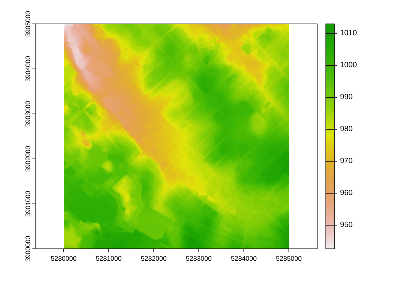
ggplot + tidyterra
ggplot()+
  geom_spatraster(data = pot_elev)+
  khroma::scale_fill_batlow()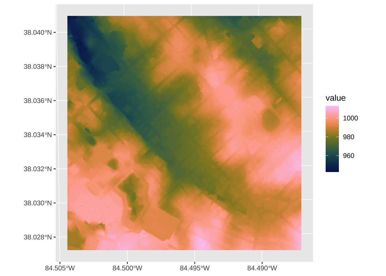
contours
ggplot()+
  geom_spatraster_contour_filled(data = pot_elev)+
  scale_fill_terrain_d()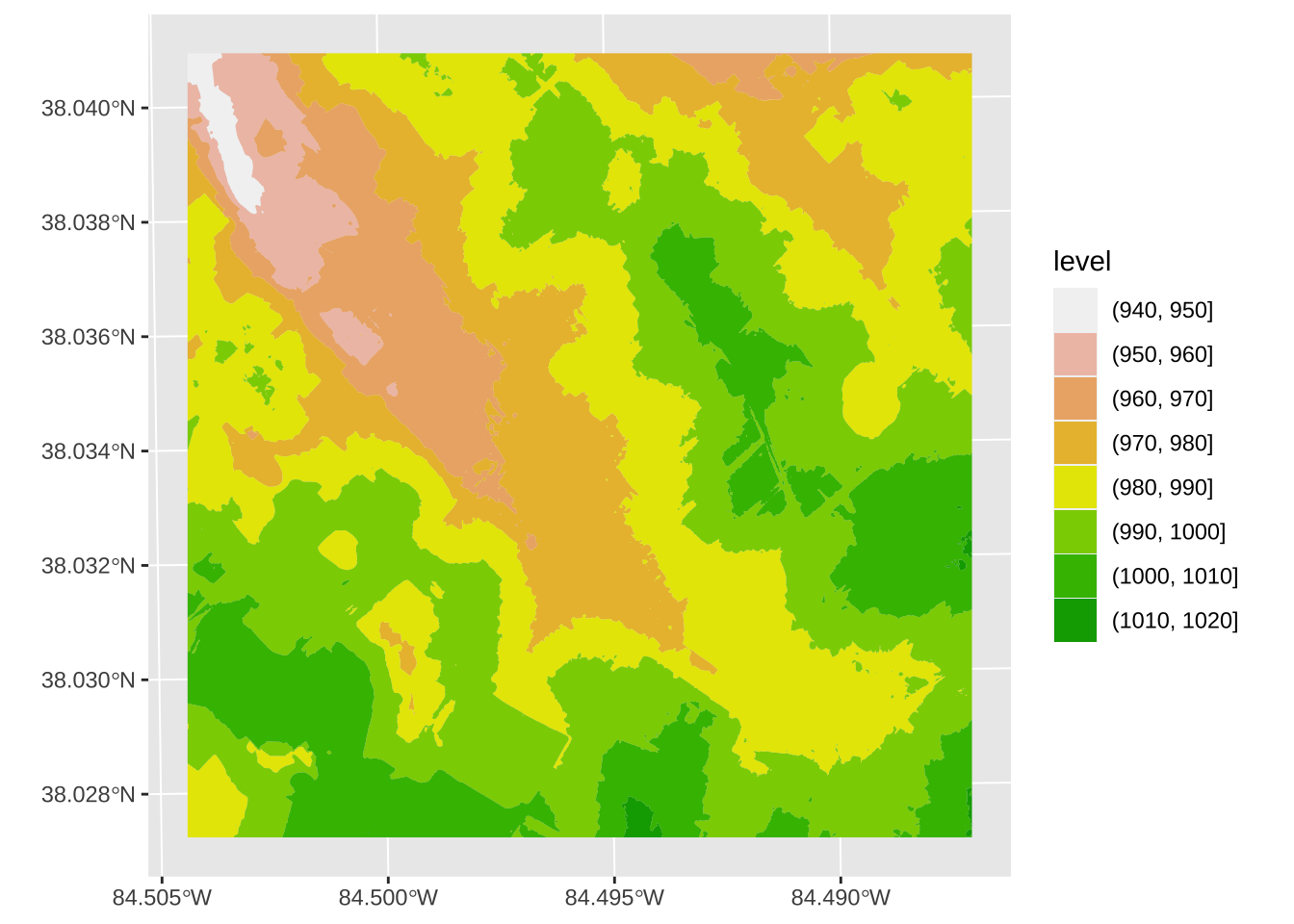
Downsampling
dim(pot_elev)[1] 2500 2500 1aggregate(pot_elev, 100)class : SpatRaster
dimensions : 25, 25, 1 (nrow, ncol, nlyr)
resolution : 200, 200 (x, y)
extent : 5280000, 5285000, 3900000, 3905000 (xmin, xmax, ymin, ymax)
coord. ref. : NAD83 / Kentucky Single Zone (ftUS) (EPSG:3089)
source(s) : memory
name : N092E301_DEM_Phase2
min value : 947.625
max value : 1010.791 ggplot() +
geom_spatraster(data = aggregate(pot_elev, 100))+
khroma::scale_fill_batlow()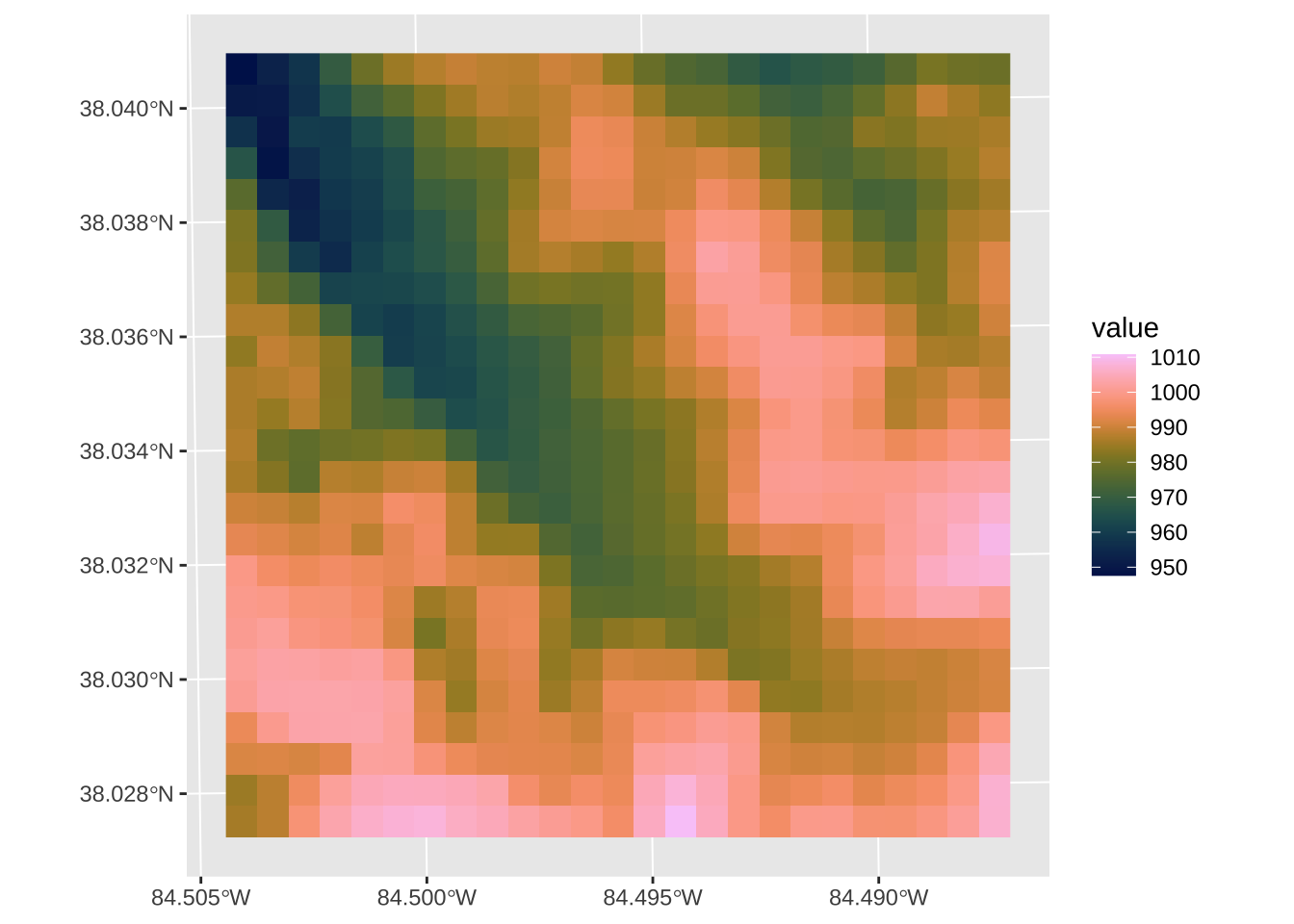
Interactions between vectors and rasters
Let’s recreate our trip to Kroger!
tribble(
~name, ~addr,
"POT", "120 Patterson Dr, Lexington, KY 40506",
"Kroger", "704 Euclid Ave, Lexington, KY 40502"
) |>
geocode(addr) |>
rowwise() |>
mutate(geom = list(st_point(c(long, lat)))) |>
st_as_sf() ->
kroger_trip
st_crs(kroger_trip) <- 4326- 1
- Setting up a dataframe of addresses to geocode.
- 2
-
From
tidygeocoder - 3
- Row-by-row, we’ll convert longitude and latitude to geographic points
- 4
- Creating the point objects
- 5
- Converting to a spatial dataframe
- 6
- Setting the coordinate reference system to the default
First, we can get the elevations of POT and Kroger, but we need to project the kroger_trip into the same crs
kroger_trip |>
st_transform(
st_crs(pot_elev)
) ->
kroger_trip- 1
-
st_transform()reprojects - 2
- We can use the crs directly from the raster object
terra::extract(pot_elev, kroger_trip) ID N092E301_DEM_Phase2
1 1 978.2686
2 2 981.7668kroger_trip |>
st_buffer(100) ->
kroger_points_100ftkroger_points_100ft |>
mapview()mask(pot_elev, kroger_points_100ft) |>
plot()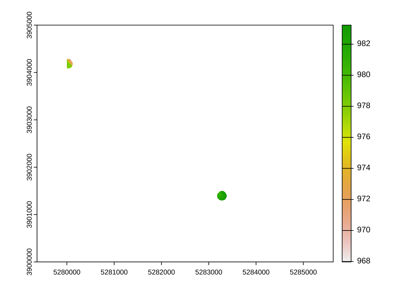
Getting our Kroger route
kroger_route <-osrmRoute(
  kroger_trip$geom[1],
  kroger_trip$geom[2],
  osrm.profile = "foot")
kroger_route |>
st_transform(st_crs(pot_elev)) |>
st_segmentize(dfMaxLength = 10) |>
st_cast("POINT") ->
route_pointsWarning in st_cast.sf(st_segmentize(st_transform(kroger_route,
st_crs(pot_elev)), : repeating attributes for all sub-geometries for which they
may not be constantterra::extract(pot_elev, route_points) -> route_elevroute_points |>
mutate(elev= route_elev$N092E301_DEM_Phase2) ->
route_point_elevggplot()+
geom_sf(data = route_point_elev, aes(color = elev))+
khroma::scale_color_batlow()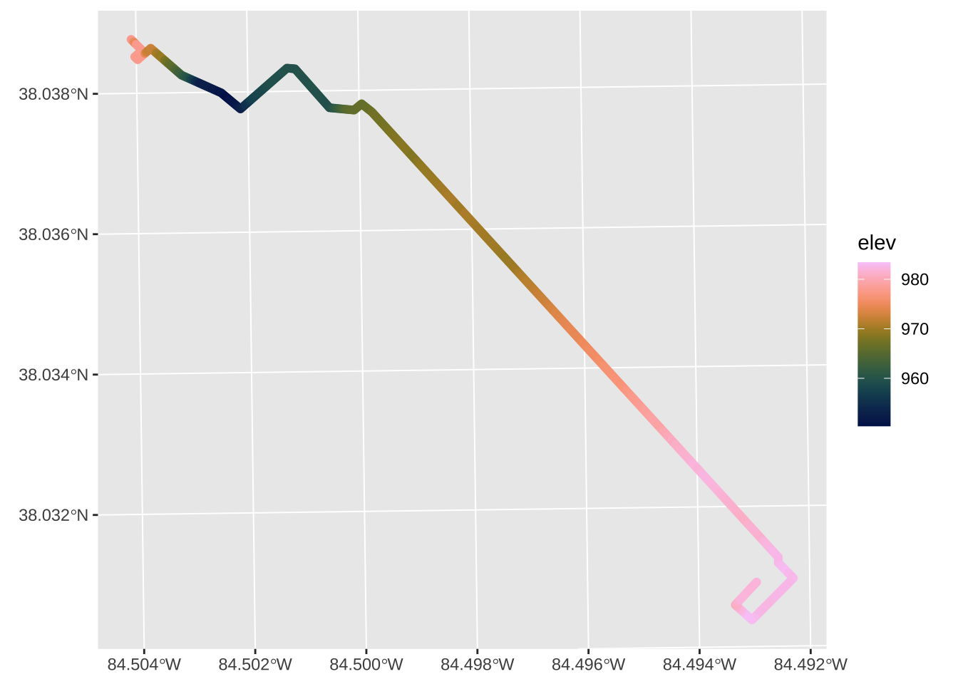
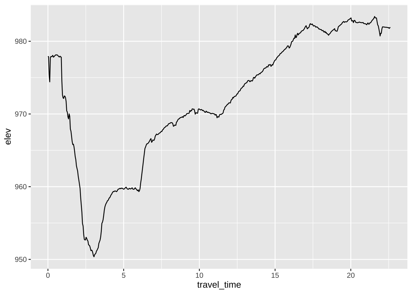
route_point_elev |>
  mutate(
    pct = seq(0, 1, length = n()),
    travel_time = duration * pct
  ) |>
  ggplot(aes(travel_time, elev))+
    geom_line()