ggplot2 extensions

There are a lot of ggplot2 extensions. You can browse some of them here:

• https://exts.ggplot2.tidyverse.org/gallery/
  

library(tidyverse)
library(palmerpenguins)
library(khroma)

Fun/eyecandy

{ggridges}

library(ggridges)

Sometimes called a “joyplot”

ggplot(drop_na(penguins), aes(x = bill_length_mm, y = species))+
    geom_density_ridges(aes(fill = species))+
    scale_fill_bright()

Picking joint bandwidth of 1.08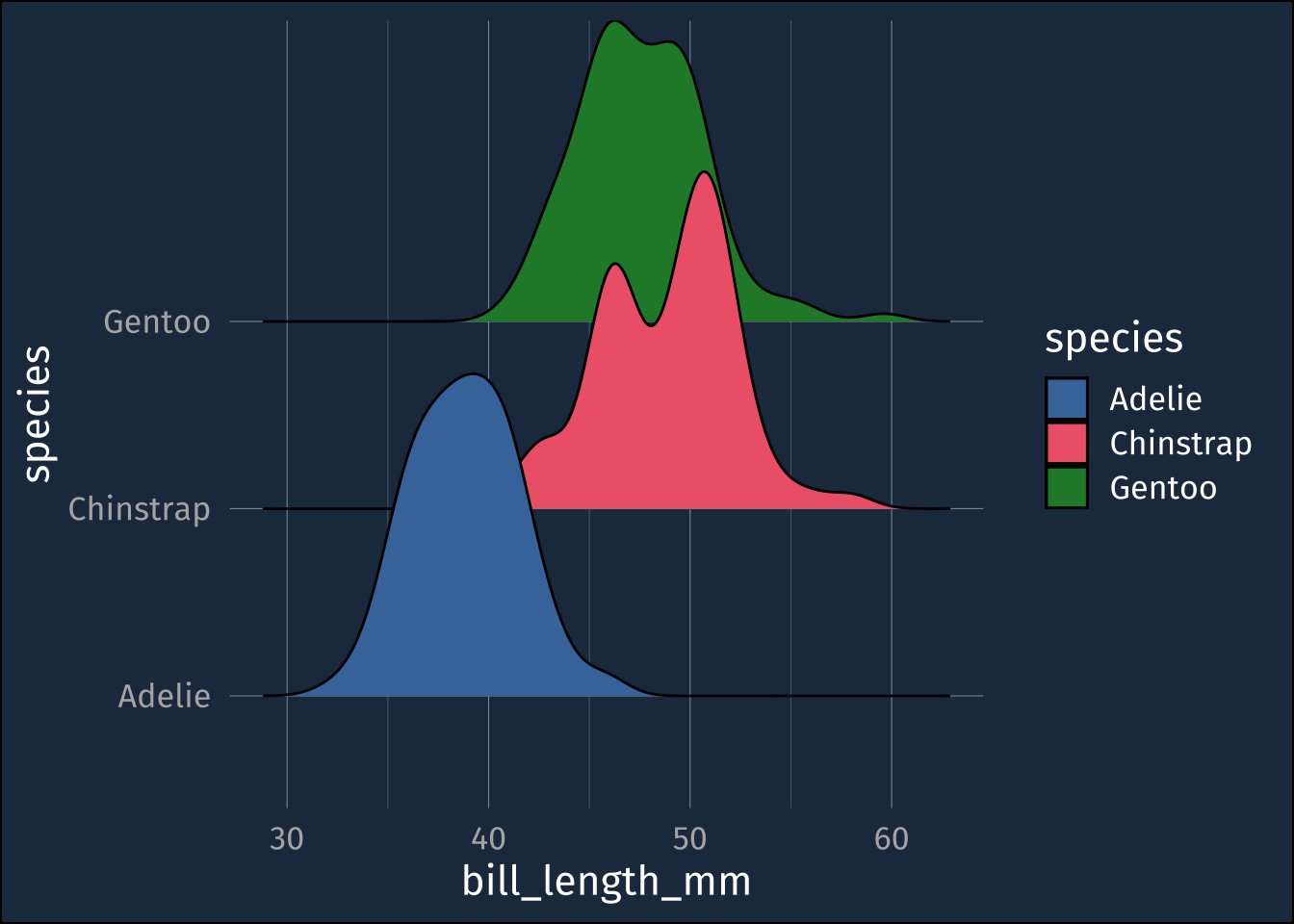

rmarkdown::paged_table(lincoln_weather)

ggplot(lincoln_weather, aes(x = `Mean Temperature [F]`, y = Month))+
  geom_density_ridges_gradient(aes(fill = after_stat(x))) +
  scale_fill_batlow()

Picking joint bandwidth of 3.37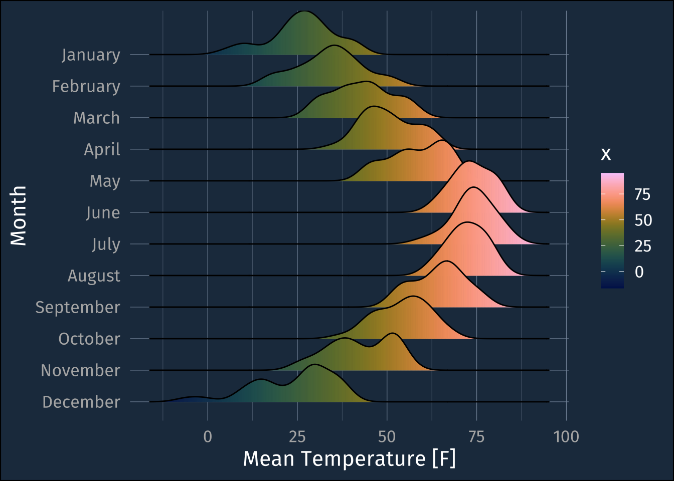

{ggpage}

library(ggpage)
library(tidytext)
library(tidyjson)

Attaching package: 'tidyjson'

The following object is masked from 'package:stats':

    filter

download.file(
  url = "https://raw.githubusercontent.com/JoFrhwld/2022_lin517/main/_site/search.json",
  destfile = "assets/search.json"
)

nlp_site <- tidyjson::read_json("assets/search.json")

We haven’t learned about stuff underneath this!

nlp_site  |>
  gather_array() |>
  hoist(..JSON,
    "title",
    "section",
    "text"
  )  |>
  as_tibble() |>
  select(array.index, title, section, text) |>
  unnest_tokens(input = text, output = "text") -> tokens_table

tokens_table 

# A tibble: 43,637 × 4
   array.index title                     section text    
         <int> <chr>                     <chr>   <chr>   
 1           1 Reading a Technical Paper ""      there   
 2           1 Reading a Technical Paper ""      may     
 3           1 Reading a Technical Paper ""      never   
 4           1 Reading a Technical Paper ""      be      
 5           1 Reading a Technical Paper ""      a       
 6           1 Reading a Technical Paper ""      point   
 7           1 Reading a Technical Paper ""      in      
 8           1 Reading a Technical Paper ""      your    
 9           1 Reading a Technical Paper ""      academic
10           1 Reading a Technical Paper ""      life    
# … with 43,627 more rows

tokens_table |> 
ggpage_build(para.fun = rpois, lambda = 75) |> 
  mutate(keywords = case_when(word == "python" ~ "python",
                              word == "probability" ~ "probability",
                              TRUE ~ "else")) |> 
  ggpage_plot(aes(fill = keywords)) +
  scale_fill_manual(values = c("grey80", "red", "blue"))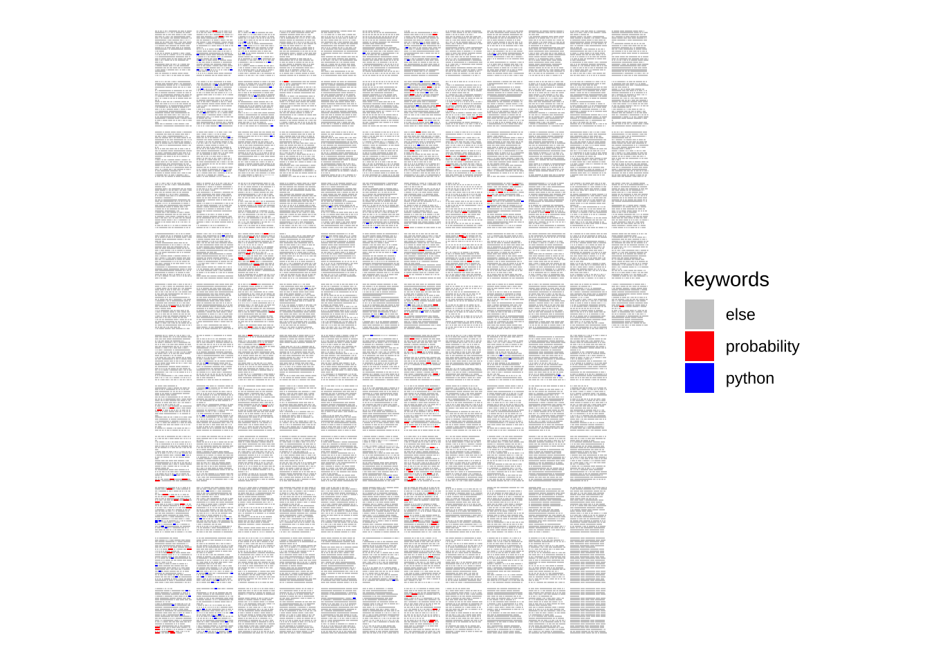

{ggbeeswarm}

Just plotting points.

ggplot(penguins, aes(species, bill_depth_mm))+
    geom_point()

Warning: Removed 2 rows containing missing values (`geom_point()`).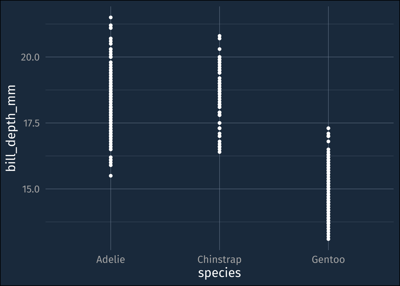

You could jitter the points.

ggplot(penguins, aes(species, bill_depth_mm))+
    geom_jitter()

Warning: Removed 2 rows containing missing values (`geom_point()`).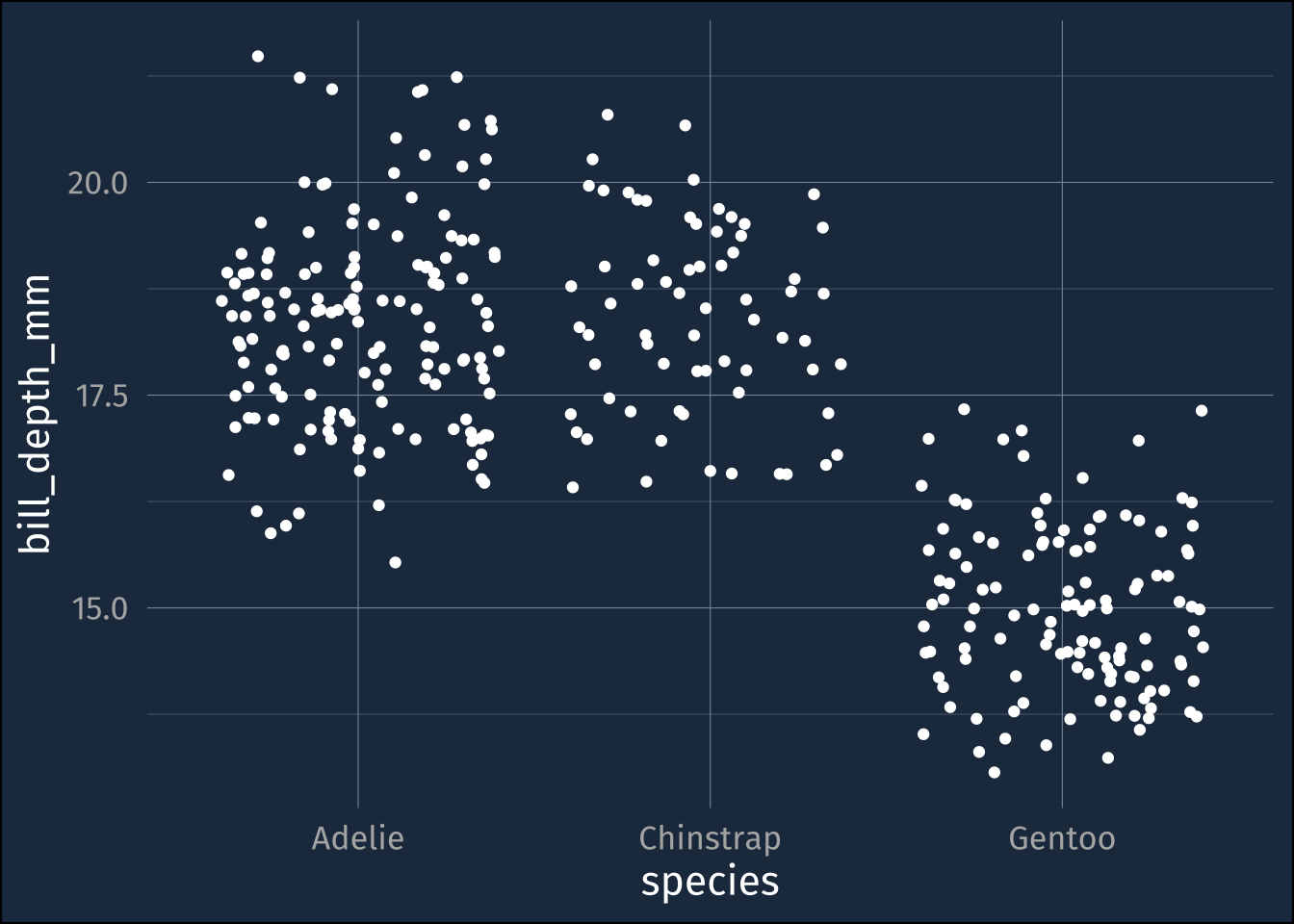

Or, you could beeswarm them

library(ggbeeswarm)

ggplot(penguins, aes(species, bill_depth_mm, color = bill_depth_mm))+
    geom_beeswarm()+
    scale_color_batlow()

Warning: Removed 2 rows containing missing values (`geom_point()`).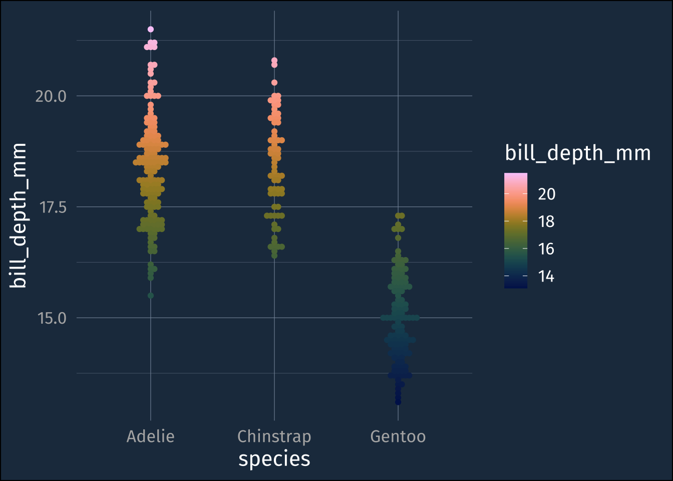

Labeling

{ggrepel}

This package tries to solve the problem of having overlapping labels on data points. If we added a text label on top of every point, chaos.

ggplot(drop_na(penguins), aes(bill_length_mm, bill_depth_mm, color = species))+
    geom_point()+
    geom_text(aes(label = island))+
    scale_color_bright()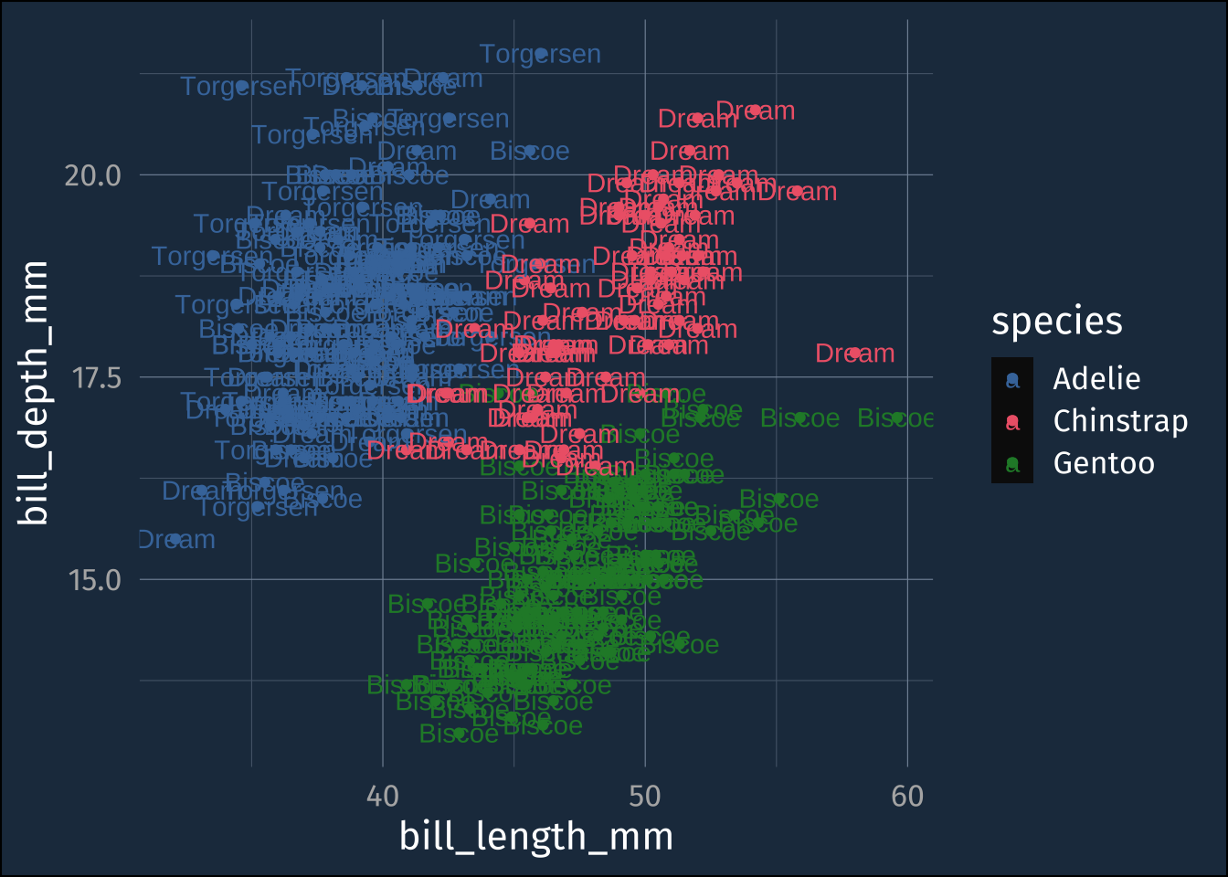

library(ggrepel)

ggplot(drop_na(penguins), aes(bill_length_mm, bill_depth_mm, color = species))+
    geom_point()+
    geom_text_repel(aes(label = island))+
    scale_color_bright()

Warning: ggrepel: 296 unlabeled data points (too many overlaps). Consider
increasing max.overlaps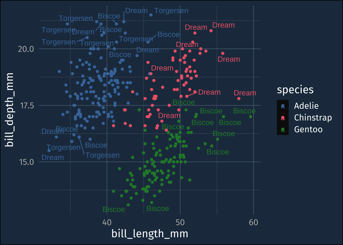

{geomtextpath}

Adds direct labels to lines

library(geomtextpath)

ggplot(penguins, aes(bill_length_mm, color = species))+
  geom_textdensity(aes(label = species))+
  scale_color_brewer(palette = "Dark2")+
  guides(
    color = "none"
  )

Warning: Removed 2 rows containing non-finite values (`stat_density()`).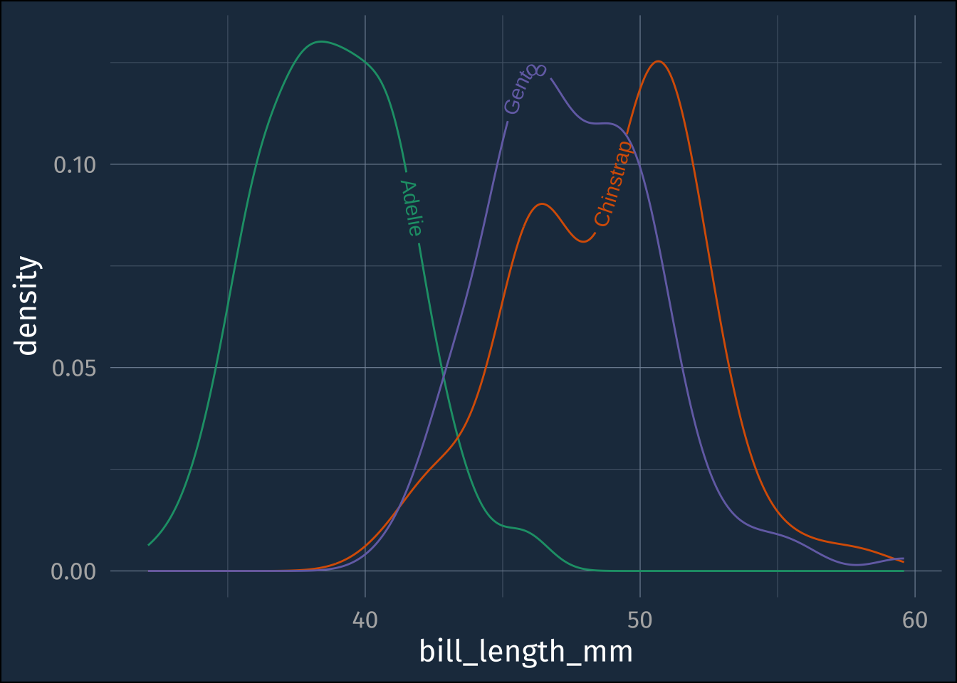

ggplot(penguins, aes(bill_length_mm, bill_depth_mm, color = species))+
    stat_ellipse(
      geom = "textpath",
      aes(label = species),
      hjust = 0.9, 
      vjust = -0.5
    )+
  guides(
    color = "none"
  )+
  scale_color_brewer(palette = "Dark2")

Warning: Removed 2 rows containing non-finite values (`stat_ellipse()`).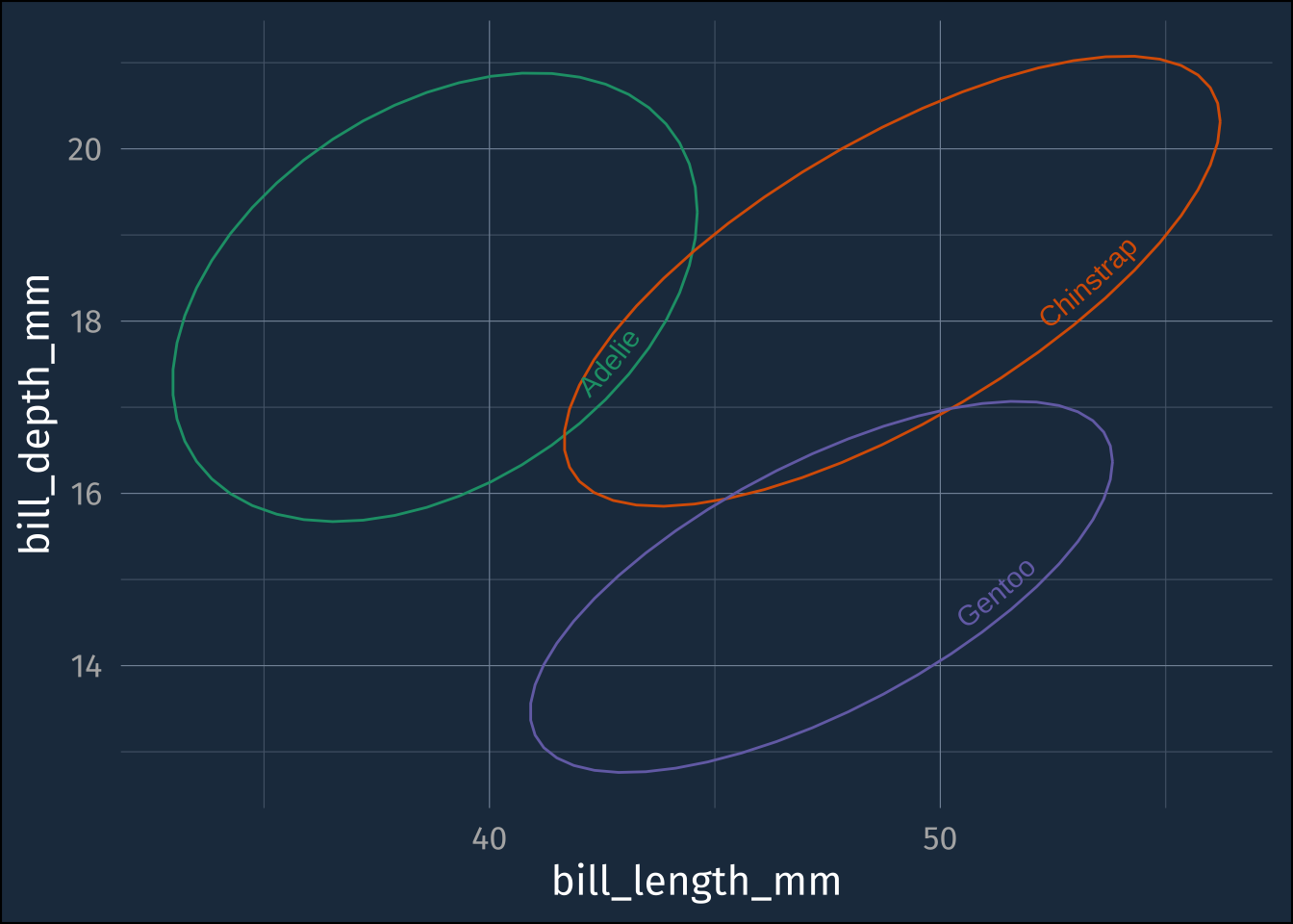

figure composition

patchwork

See also https://ggplot2-book.org/arranging-plots.html

library(patchwork)
library(ggdensity)

depth_plot <- ggplot(penguins, aes(bill_depth_mm, color = species))+
  geom_textdensity(aes(label = species))+
  coord_flip()+
  scale_color_brewer(palette = "Dark2")

length_plot <- ggplot(penguins, aes(bill_length_mm, color = species))+
  geom_textdensity(aes(label = species))+
  scale_color_brewer(palette = "Dark2")

(depth_plot | length_plot) + plot_layout(guides = "collect")

Warning: Removed 2 rows containing non-finite values (`stat_density()`).
Removed 2 rows containing non-finite values (`stat_density()`).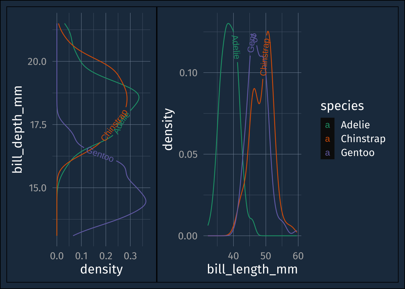

(depth_plot | length_plot) + plot_layout(guides = "collect")

Warning: Removed 2 rows containing non-finite values (`stat_density()`).
Removed 2 rows containing non-finite values (`stat_density()`).

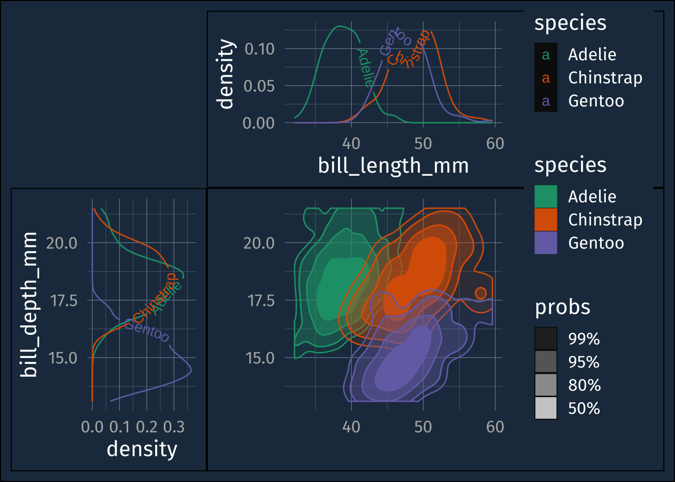
scatter <-
  ggplot(penguins, aes(bill_length_mm, bill_depth_mm, color = species))+
    stat_hdr(aes(fill = species))+
    scale_fill_brewer(palette = "Dark2")+
    scale_color_brewer(palette = "Dark2")+
    theme(
      axis.title = element_blank()
    )
scatter

Warning: Removed 2 rows containing non-finite values (`stat_hdr()`).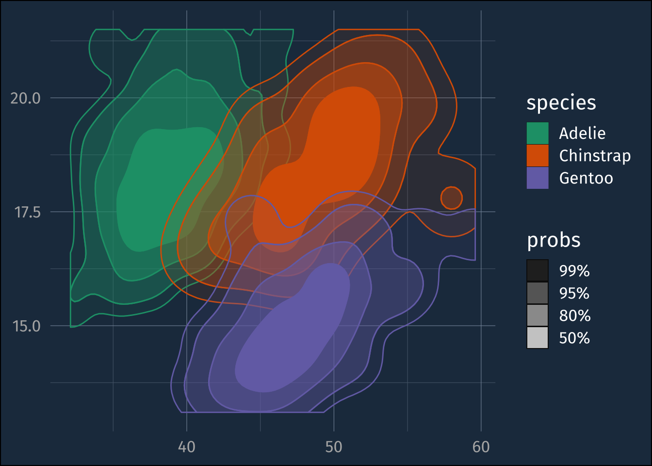

This could use some work, but it’s on its way

layout <- "
#AA
BCC
BCC
"
length_plot + depth_plot + scatter + plot_layout(design = layout, guides = "collect")

Warning: Removed 2 rows containing non-finite values (`stat_density()`).
Removed 2 rows containing non-finite values (`stat_density()`).

Warning: Removed 2 rows containing non-finite values (`stat_hdr()`).