Statistical Rethinking Workthrough Blog - Where I do a lot of work and don’t understand colliders any better.

Listening

Setup

Code

library(tidyverse)
library(tidybayes)
library(brms)
library(gt)
library(gtsummary)
library(patchwork)
library(ggblend)
library(ggdensity)
library(ggforce)
library(marginaleffects)
library(dagitty)
library(ggdag)
library(khroma)


source(here::here("_defaults.r"))

set.seed(2023-9-7)

Developing a sense for colliders

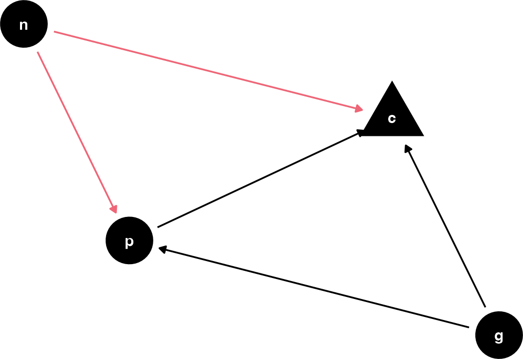
For me to really get a sense of how coliders work, I’m going to have to simulate a few different datasets, messing around with the parameters, and compare the outcomes. I won’t do this full Bayesian for the sake of speed. As a reminder, here’s the DAG. I’ll specifically be messing around with the effect of n on p and c.

Code

dagify(
  c ~ p + g + n,
  p ~ g + n
) |> 
  tidy_dagitty() ->
  the_dag

the_dag |> 
  mutate(
    from_n = ifelse(name == "n", ptol_red, "black")
  ) |> 
  ggplot(aes(x = x, y = y, xend = xend, yend = yend)) +
    geom_dag_point(
      aes(
        shape = name == "c"
      )
    )+
    geom_dag_edges(
      aes(
        edge_color = from_n
      )
    )+
    geom_dag_text()+
    scale_color_manual(
      values = c("grey60", ptol_red)
    )+
    guides(
      shape = "none",
      color = "none"
    )+
    theme_dag()

I refactored the code from before into a function:

simulation function

sim_collider <- function(
    n = 200,
    # Grandparent on parent
    b_GP = 1,
    # Parent on Child
    b_PC = b_GP,
    # Grandparent on Child
    b_GC = 0,
    # neighborhood
    b_N = 2){
  
  tibble(
    grandparent = rnorm(n),
    neighborhood = rbinom(
      n, 
      size = 1, 
      prob = 0.5
    ),
    parent = rnorm(
      n,
      mean = b_GP * grandparent + 
        b_N * neighborhood
    ),
    child = rnorm(
      n,
      mean = b_GC * grandparent +
        b_PC * parent + 
        b_N  * neighborhood
    )
  ) ->
    haunted_sim
  
  return(haunted_sim)
}

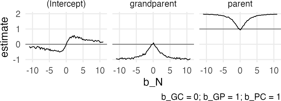
And I’ll do a grid of 100 values from -11 to 11 for b_N.

simulation parameters

tibble(
  n = 200,
  b_GP = 1,
  b_PC = 1,
  b_GC = 0,
  b_N = rep(seq(-11, 11, length = 100), 10)
) -> 
  sim_params

Now, with some tidyverse fanciness, I’ll map the simulation function I wrote across each row to get simulation datasets.

Simulating the data with pmap

sim_params |> 
  rowwise() |> 
  mutate(
    data = pmap(
      list(n, b_GP, b_PC, b_GC, b_N),
      sim_collider
    )
  ) |> 
  ungroup()->
  sim_data

Then, for each data set I’ll fit

lm(child ~ parent + grandparent)

and then get the parameters.

Fitting a model for each simulation

sim_data |> 
  mutate(
    model = map(
      data, 
      ~lm(child ~ parent + grandparent, data = .x)
    ),
    params = map(model, broom::tidy)
  ) |> 
  unnest(params) |> 
  select(
    starts_with("b_"),
    term, 
    estimate
  ) ->
  model_params

Code

true_params <- tibble(
  term = c("(Intercept)", "grandparent", "parent"),
  estimate = c(0, 0, 1)
)

model_params |> 
  ggplot(
    aes(
      b_N,
      estimate
    )
  )+
  geom_hline(
    data = true_params,
    aes(
      yintercept = estimate
    ),
    color = "grey40"
  )+
  stat_summary(
    fun.y = mean,
    geom = "line"
  )+
  facet_wrap(~term)+
  labs(
    caption = "b_GC = 0; b_GP = 1; b_PC = 1"
  )

Huh. I guess I wasn’t expecting an asymptotic relationship for the grandparent and parent effects? It looks like as b_N gets large, the collider confounding reaches some kind of min/max, which for grandparent is -1, and for parent is 1. I don’t know if this value relates to either the effect of b_GP or b_PC, since both were set to 1? Maybe time for another grid search. I’ll really max outt the b_N effect to get fully into the tail of the asymptote.

One big simulation

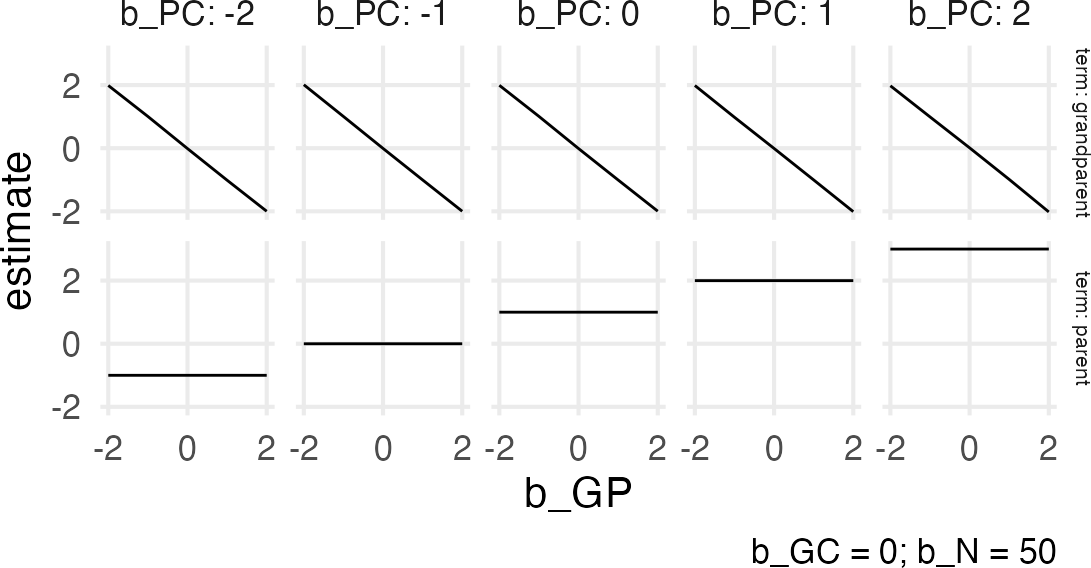
expand_grid(
  n = 200,
  b_GP = rep(-2:2, 10),
  b_PC = rep(-2:2, 10),
  b_GC = 0,
  b_N = 50
) |> 
  rowwise() |> 
  mutate(
    data = pmap(
      list(n, b_GP, b_PC, b_GC, b_N),
      sim_collider
    )
  ) |> 
  ungroup() |> 
  mutate(
    model = map(
      data, 
      ~lm(child ~ parent + grandparent, data = .x)
    ),
    params = map(model, broom::tidy)
  ) |> 
  unnest(params) |> 
  select(
    starts_with("b_"),
    term, 
    estimate
  ) ->
  big_sim

Code

big_sim |> 
  filter(
    term != "(Intercept)"
  ) |> 
  ggplot(
    aes(
      b_GP,
      estimate
    )
  )+
    stat_summary(
      fun.y = mean,
      geom = "line"
    )+
    scale_x_continuous(
      breaks = c(-2, 0, 2)
    )+
    scale_y_continuous(
      breaks = c(-2, 0, 2)
    )+
    facet_grid(term~b_PC, labeller = label_both)+
    theme(
      aspect.ratio = 1,
      strip.text.y  = element_text(size = 8)
    )+
    labs(
      caption = "b_GC = 0; b_N = 50"
    )

Huh. The associations look straightforward, but I think I need an animation to get it.

This turned into a whole thing.

Code

library(gganimate)
nframes = 100

Code

color_value <- function(x, min.v = -2, max.v = 2, scale = color("berlin")(100)){
  prop = (x - min.v)/(max.v-min.v)
  closest_idx = round(prop * (length(scale)-1))+1
  return(scale[closest_idx])
}

Code

tibble(
  name = "p",
  to = "c",
  true = 1,
  est = true + 1,
  id = seq(-2, 2, length = nframes),
  col = color_value(true)
) |> 
  bind_rows(
    tibble(
      name = "g",
      to = "c",
      true = 0,
      est = seq(2, -2, length = nframes),
      id = seq(-2, 2, length = nframes),
      col = color_value(true)
    )
  ) |> 
  bind_rows(
    tibble(
      name = "g",
      to = "p",
      true = seq(-2, 2, length = nframes),
      est = NA ,
      id = seq(-2, 2, length = nframes),
      col = color_value(true)
    )
  ) |> 
  bind_rows(
    tribble(
      ~name, ~to, ~true, ~est,
     "n", "c",  NA,  NA,
     "n", "p",  NA,  NA,
     "c", NA, NA, NA
    ) |> 
      mutate(
        across(true:est, as.numeric),
        col = "#000000"
      ) |> 
      group_by(name, to, true, est, col) |> 
      reframe(
        id = seq(-2, 2, length = nframes)
      ) 
  )->
  pc_true_anim

tibble(
  name = "p",
  to = "c",
  true = 1,
  est = true + 1,
  id = seq(-2, 2, length = nframes),
  col = color_value(est)
) |> 
  bind_rows(
    tibble(
      name = "g",
      to = "c",
      true = 0,
      est = seq(2, -2, length = nframes),
      id = seq(-2, 2, length = nframes),
      col = color_value(est)
    )
  ) ->
  pc_est_anim

Code

pc_true_anim |> 
  left_join(the_dag |> as_tibble()) ->
  true_dag

pc_est_anim |> 
  left_join(the_dag |> as_tibble()) ->
  est_dag

Code

true_dag |> 
  ggplot(aes(x = x, y = y, xend = xend, yend = yend)) +
    geom_dag_point(
      color = "grey",
    )+
    geom_dag_text()+
    geom_segment(
      arrow = arrow(type = "closed", length = unit(0.2, "cm")),
      linewidth = 1,
      aes(
        color = col
      )
    )+
    geom_segment(
      data = est_dag,
      linetype = "dashed",
      aes(
        x = x+0.1, y = y+0.1, xend = xend+0.1, yend = yend+0.1,
        color = col
      ),
      arrow = arrow(type = "closed", length = unit(0.2, "cm")),
      linewidth = 1
    )+
    scale_color_identity()+
    transition_time(
      id
    )+
  labs(
    title = "b_GP: {round(frame_time, digits = 2)}\nest_GC: {round(frame_time*-1, digits = 2)}"
  )+
  theme_dag()->a
animate(a, rewind = T) |> 
  anim_save(
    filename = "dag_anim.gif"
  )

So, as the true effect of Grandparents on parents changes, the estimated direct effect on children is inversely proportional, and, for some reason, the direct effect of parents is just +1?