Let’s try some summaries. For the categorical data, I’m going to do my own custom summary, but for the numeric columns I’ll just use gtsummary::tbl_summary().
As it turns out, just like usual when I start trying to finesse things, the code got a little intense.
Categorical summary
milk |>select(where(~!is.numeric(.x) ) ) |>pivot_longer(cols =everything(),names_to ="var",values_to ="value" ) |>summarise(.by = var,total_groups =n_distinct(value),most_common =fct_count(factor(value),sort = T,prop = T ) |>slice(1) ) |>unnest(most_common) |>gt() |>cols_label(var ="Variable",total_groups ="Total Groups",f ="Most common",n ="Number of most common",p ="Proportion of most common" ) |>fmt_number(columns = p,decimals =2 )
Variable
Total Groups
Most common
Number of most common
Proportion of most common
clade
4
Ape
9
0.31
species
29
A palliata
1
0.03
Table 1:
Summary of categorical variables
Comparing the code I wrote for the categorical variables to how straightforward tbl_summary() is kind of illustrates how useful these out-of-the-box tools can be.
milk |>select(where(is.numeric) ) |>tbl_summary()
Characteristic
N = 291
kcal.per.g
0.60 (0.49, 0.73)
perc.fat
37 (21, 46)
perc.protein
15.8 (13.0, 20.8)
perc.lactose
49 (38, 60)
mass
3 (2, 11)
neocortex.perc
68.9 (64.5, 71.3)
Unknown
12
1 Median (IQR)
Table 2:
Summary of continuous variables
The initial model
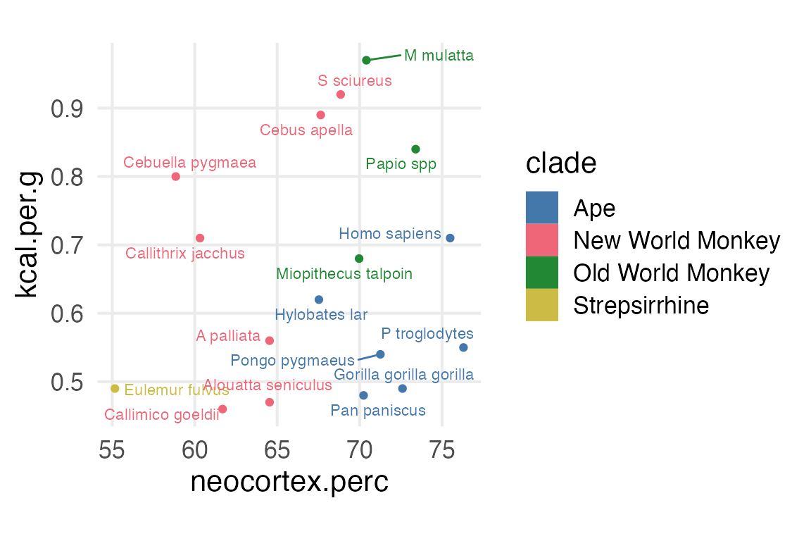
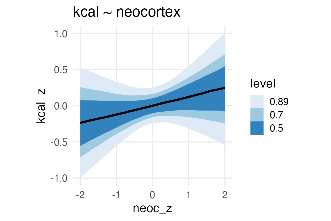
Ok, we’re going to model the kilocalories per gram of milk as the outcome, trying to explore whether or not the neocortex percentage is related.
Figure 1: Neorcortex percentage and kcal per gram of milk
Preparing the data
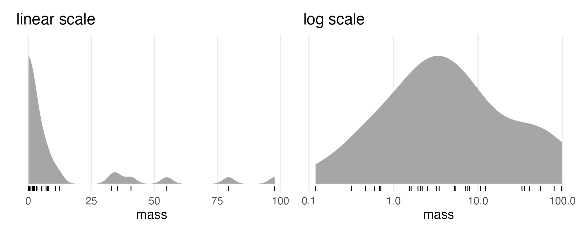
I won’t look ahead and drop NAs when I standardize to save some space. Looks like we’re logging the body mass. I’ll just check that distribution real quick.
I’ll fit models with both the weak priors and the stronger priors. I’m still needing to check what everything is called with get_prior() before I can confidently set anything.
get_prior( kcal_z ~ neoc_z,data = milk_to_mod)
                   prior     class   coef group resp dpar nlpar lb ub
                  (flat)         b
                  (flat)         b neoc_z
 student_t(3, -0.2, 2.5) Intercept
    student_t(3, 0, 2.5)     sigma                               0
       source
      default
 (vectorized)
      default
      default
Ok, should do the trick.
brm( kcal_z ~ neoc_z,data = milk_to_mod,prior =c(prior(normal(0,1), class = b),prior(normal(0,1), class = Intercept),prior(exponential(1), class = sigma) ),sample_prior = T,file ="neoc_model_weak.rds",cores =4,backend ="cmdstanr")-> neoc_model_weak
brm( kcal_z ~ neoc_z,data = milk_to_mod,prior =c(prior(normal(0,0.5), class = b),prior(normal(0,0.2), class = Intercept),prior(exponential(1), class = sigma) ),sample_prior = T,file ="neoc_model_strong.rds",cores =4,backend ="cmdstanr")-> neoc_model_strong
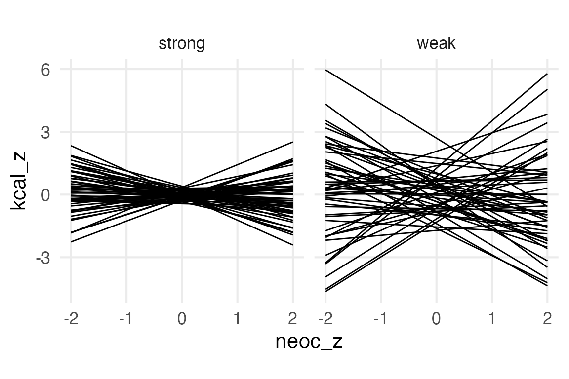
Prior predictive plots
You can set an option in brm to only sample the priors for something like this, but instead I just fit whole models to save time. This’ll need to be a bit “manual”, cause I don’t think marginaleffects::predictions() has an option to get prior predictions.
So, the “weaker” priors are “silly” (as McElreath puts it) because for some noec_z values, it’s predicting kcal_z values as extreme as 6. And because I standardized the outcome, that’s saying some kcal_z values are up to 6 standard deviations from the average. R actually craps out trying to give the cumulative probability!
pnorm(6, mean =0, sd =1)
[1] 1
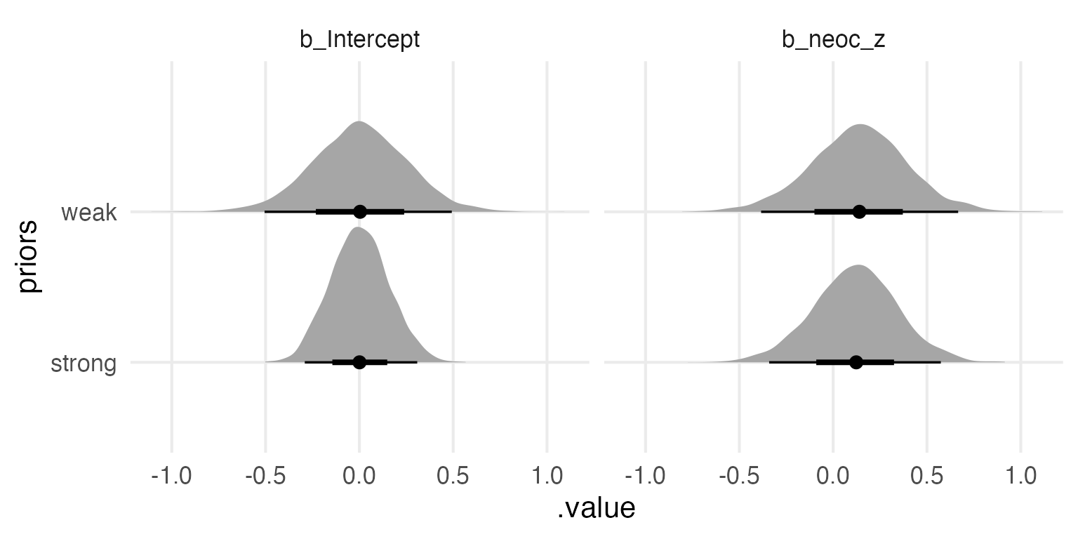
The Posteriors
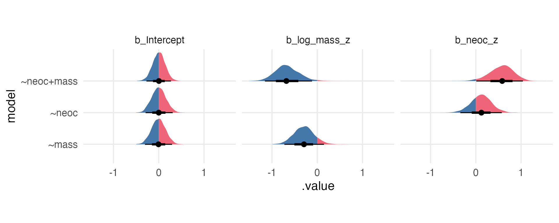
Lemme compare the posterior parameter estimates for the two models.
neoc_model_weak |>gather_draws(`b_.*`,regex = T ) |>mutate(priors ="weak") -> weak_betasneoc_model_strong |>gather_draws(`b_.*`,regex = T ) |>mutate(priors ="strong") -> strong_betas
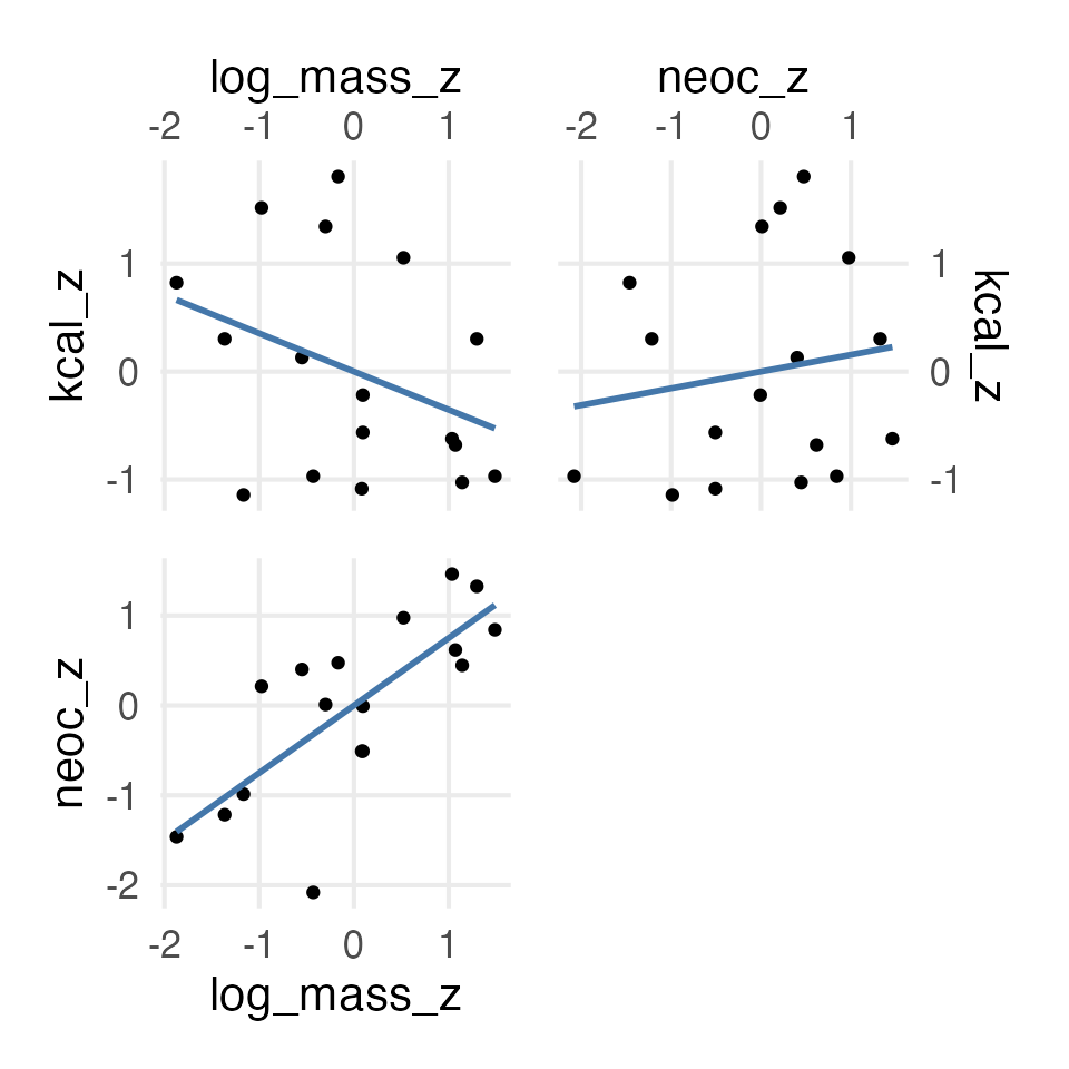
Figure 9: Relationship between the three variables
Isn’t this collinearity?
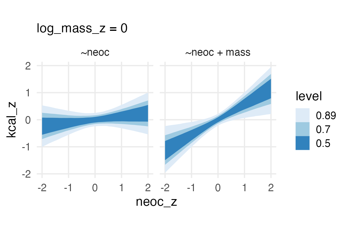
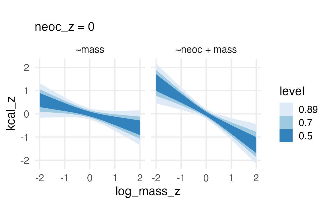
So, on this point, I’m not completely sure how I should feel about the model with both body mass and neocortex percentage, since it looks like “collinearity” which is supposed to be 👻 spooky 👻. In the book, he gives three possible DAGs, so I’ll see what the “adjustment sets” are like for each.
Well, they all say to get the direct effect of neocortex percentage on kcal per gram, you need to include mass… Which I can be cool with, I just need to figure out how we’re thinking about collinearity now! Maybe the paper Collinearity isn’t a disease that needs curing is a place to start!