Statistical Rethinking Workthrough Blog

Listening

Setup

Code

library(tidyverse)
library(tidybayes)
library(brms)
library(gt)
library(gtsummary)
library(patchwork)
library(ggblend)
library(ggdensity)
library(ggforce)
library(marginaleffects)
library(dagitty)
library(ggdag)


source(here::here("_defaults.r"))

set.seed(2023-9-6)

Collider Bias

When A has an effect on Z, and B has an effect on Z, then Z is a “collider” variable between A and B.

graph LR
  a["A"]
  b["B"]
  z["Z"]
  
  a --> z
  b --> z

So, if I understand things right, fitting a model with

A ~ B

would result in no effect of B on A, which we can check with a DAG.

dagify(
  Z ~ A,
  Z ~ B
) |> 
  impliedConditionalIndependencies()

A _||_ B

But, if we fit a model with

A ~ B + Z

now there would suddenly seem to be an effect of B on A. As a simple demo, we can repeat the simulation of newsworthiness and trustworthiness.

simulating selection

tibble(
  trustworthiness = rnorm(200),
  newsworthiness = rnorm(200),
  score = trustworthiness + newsworthiness,
  score_percentile = ecdf(score)(score),
  selected = score_percentile >= 0.9
) ->
  research

Code

research |> 
  ggplot(
    aes(
      newsworthiness,
      trustworthiness,
      color = selected
    )
  ) +
    geom_point()+
    theme(
      aspect.ratio = NULL
    )+
    coord_fixed()

Last time we just fit a model using the subset of selected values. But here it goes modelling with the whole dataset. First, without the collider.

no collider model

brm(
  trustworthiness ~ newsworthiness,
  data = research,
  backend = 'cmdstanr',
  file = "research1"
)->
  research1_mod

Then, with the collider.

collider model

brm(
  trustworthiness ~ newsworthiness + selected,
  data = research,
  backend = 'cmdstanr',
  file = "research2"
)->
  research2_mod

getting parameters

list(
  `no collider` = research1_mod,
  collider = research2_mod
) |> 
  map(
    ~.x |> 
      gather_draws(
        `b_.*`,
        regex = T
      )
  ) |> 
  list_rbind(
    names_to = "model"
  )->
  collide_comp

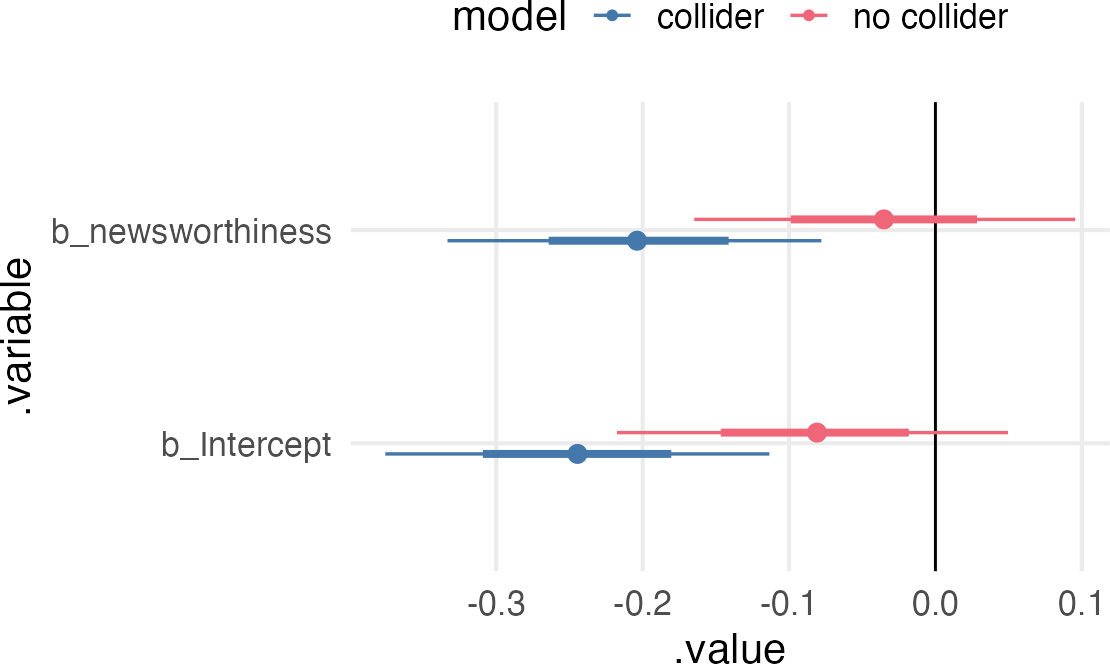
Just focusing on the intercept and newsworthiness effects, they went from (correctly) being unrelated in the model without the collider, to having pretty reliable effects by just including the selected variable.

Code

collide_comp |> 
  filter(
    str_detect(
      .variable,
      "selected",
      negate = T
    )
  ) |> 
  ggplot(
    aes(
      .value,
      .variable,
      color = model
    )
  ) +
    geom_vline(xintercept = 0) +
    stat_pointinterval(
      position = position_dodge(width = 0.2)
    )+
    theme(legend.position = "top")

Figure 2: Comparing estimates from models with and without the collider

Haunting!

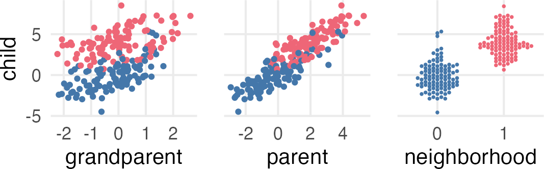
Here’s the scary part. The illustration from the book is about inter-generational effects on education. Grandparents will have an effect on their children (the parent) and parents will have an effect on their children. The question is, is there any direct effect of grandparents on children.

graph LR
  g[Grandparent]
  p[Parent]
  c[Child]
  
  g --> p
  g -.->|?| c
  p --> c

finding the direct effect

dagify(
  p ~ g,
  c ~ p,
  c ~ g
) |> 
  adjustmentSets(
    exposure = "g", 
    outcome = "c",
    effect = "direct"
  )

{ p }

Ok, but the spooky thing is what if there’s a variable (like, neighborhood) that’s shared by the parent and child, but not the grandparent, which we didn’t record.

graph LR
  g[Grandparent]
  p[Parent]
  c[Child]
  n[Neighborhood]
  
  g -.->|?| c
  g --> p
  p --> c
  n --> p
  n --> c
  
  style n stroke-dasharray: 5 5

Parent has apparently become a collider, but I’m still trying to noodle through why.

Ok, having stepped away for a bit, I think my problem was some confusion about how the “paths” work in DAGs.

I realized:

The connections from one node to another are directed.
But when charting a path from a variable to the outcome, you ignore the directedness.
Then, you add back in the directedness to diagnose confounder, mediator, collider etc.

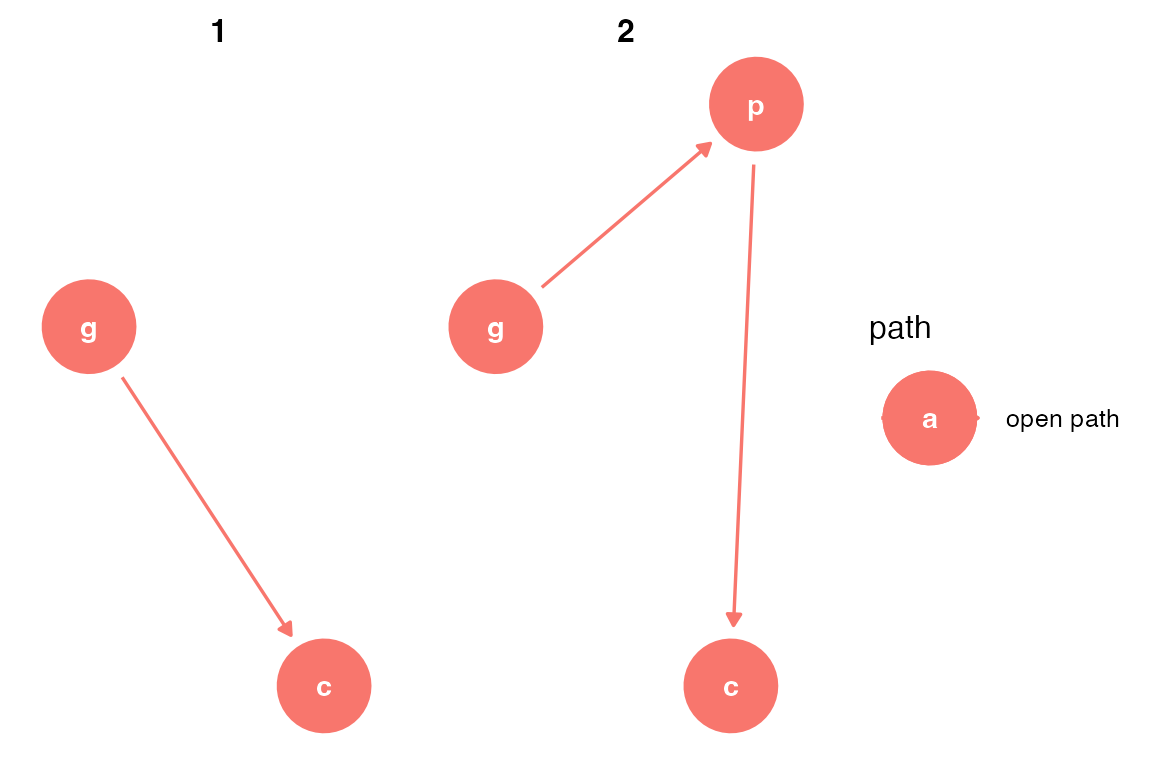
So, ignoring the directedness, we have the following paths from Grandparent to Child.

Undirected Paths

Grandparent — Child
Grandparent — Parent — Child
Grandparent — Parent — Neighborhood — Child

Then, we can add in the directedness

Directed Paths

Grandparent → Child
Grandparent → Parent → Child
Grandparent → Parent ← Neighborhood → Child

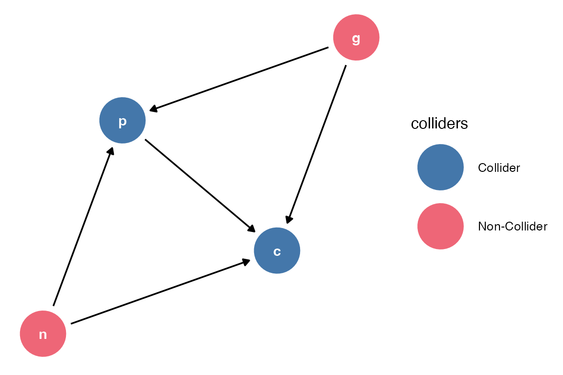
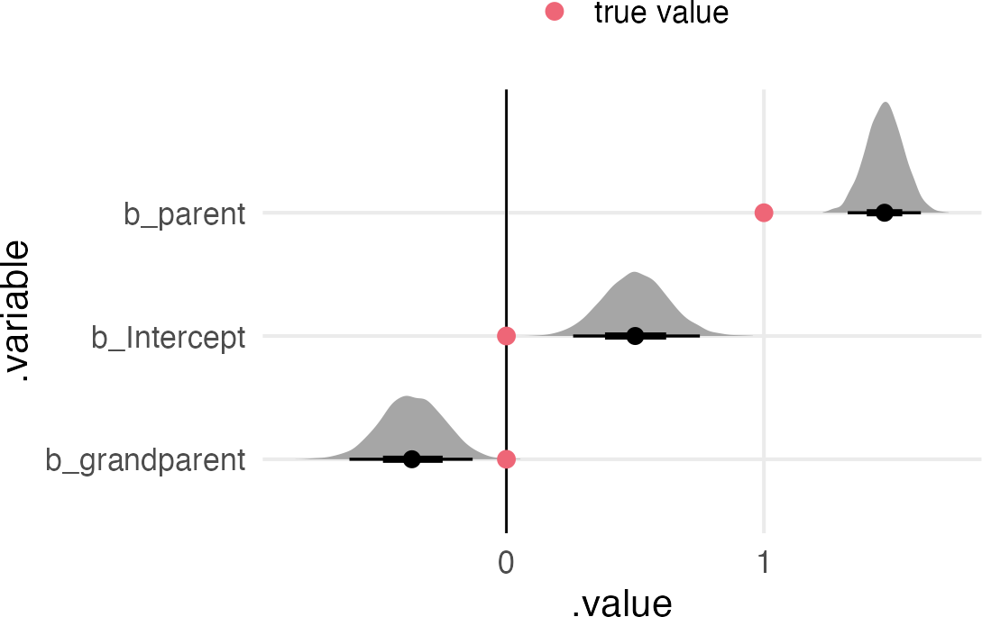
Because of path 2, (Grandparent → Parent → Child), in order to get the “direct effect” of Grandparent, we need to include Parent. But because of path 3 (Grandparent → Parent ← Neighborhood → Child), Parent is also a Collider. If we don’t include Neighborhood in the model (maybe because we didn’t measure it!) the estimate for Grandparent is going to get all screwy!

I’m still developing my intuitions for why and how the estimate will get screwy.

Getting the paths

With {dagitty} and {ggdag} you’re supposed to be able to get the paths automatically, but I can’t get the {ggdag} one to work give me the collider path.

making the dag

dagify(
  c ~ g + p + n,
  p ~ g + n
) ->
  haunted_dag

with dagitty

haunted_dag |> 
  paths(
    from = "g",
    to = "c"
  ) |> 
  pluck("paths")

[1] "g -> c"           "g -> p -> c"      "g -> p <- n -> c"

with ggdag

haunted_dag |> 
  ggdag_paths(
    from = "g",
    to = "c",
    directed = F
  )+
    theme_dag()

I think ggdag::ggdag_paths() is calling dagitty::paths() underneath, and just isn’t passing the directed argument correctly as of

Sys.Date()

[1] "2023-09-06"

I can get it to plot colliders, though.

haunted_dag |> 
  ggdag_collider()+
  theme_dag()

Simulating the haunted dag

I’ll mostly just copy the simulation parameters from the book.

setting the direct effects

# Grandparent on parent
b_GP <- 1

# Parent on Child
b_PC <- b_GP

# Grandparent on Child
b_GC <- 0

# neighborhood
b_N <- 2

The simulation

n = 200

tibble(
  grandparent = rnorm(n),
  neighborhood = rbinom(
    n, 
    size = 1, 
    prob = 0.5
  ),
  parent = rnorm(
    n,
    mean = b_GP * grandparent + 
           b_N * neighborhood
  ),
  child = rnorm(
    n,
    mean = b_GC * grandparent +
           b_PC * parent + 
           b_N  * neighborhood
  )
) ->
  haunted_sim

Code

haunted_sim |> 
  ggplot(
    aes(
      grandparent,
      child,
      color = factor(neighborhood)
    )
  )+
  geom_point()+
  guides(
    color = "none"
  )+
  theme(
    aspect.ratio = 0.8
  )->
  gc_plot

haunted_sim |> 
  ggplot(
    aes(
      parent,
      child,
      color = factor(neighborhood)
    )
  )+
    geom_point()+
  theme_blank_y()+
  guides(
    color = "none"
  )+  
  theme(
    aspect.ratio = 0.8
  )->  
  pc_plot

haunted_sim |> 
  ggplot(
    aes(
      factor(neighborhood),
      child,
      fill = factor(neighborhood),
      color = factor(neighborhood)
    )
  )+
    geom_dots(
      dotsize = 1.3,
      layout = "hex",
      side = "both"
    )+
  labs(x = "neighborhood")+
  theme_blank_y()+
  guides(
    color = "none",
    fill = "none"
  )+  
  theme(
    aspect.ratio = 0.8
  )->
  nc_plot

gc_plot + pc_plot + nc_plot

Now, let’s fit the model with just grandparent and parent (because, in this example, we don’t know about the neighborhood).

the haunted collider model

brm(
  child ~ parent + grandparent,
  data = haunted_sim,
  prior = c(
    prior(normal(0,3), class = b)
  ),
  backend = "cmdstanr",
  cores = 4,
  file = "haunted1"
)->
  haunted1_mod

Now let’s get the parameters and compare them to the true values that we created the simulation with.

true values

tribble(
  ~.variable, ~.value,
  "b_Intercept", 0,
  "b_grandparent", b_GC,
  "b_parent", b_PC
)->
  true_param

haunted params

haunted1_mod |> 
  gather_draws(
    `b_.*`,
    regex = T 
  ) ->
  haunted1_params

Code

haunted1_params |> 
  ggplot(
    aes(
      .value,
      .variable
    )
  ) +
    geom_vline(xintercept = 0)+
    stat_halfeye()+
    geom_point(
      data = true_param,
      aes(color = "true value"),
      size = 3
    )+
    scale_color_manual(
      values = ptol_red,
      name = NULL
    )+
    theme(
      legend.position = "top"
    )

As far as things go, the model will make good predictions, because the statistical associations are correct, but the causal interpretation (“Grandparents have a negative effect”) is wrong.

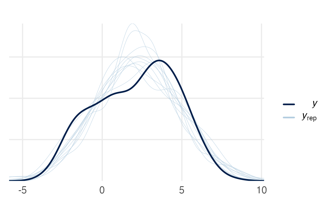
posterior predictive check

pp_check(haunted1_mod)

Figure 5: Haunted posterior predictive check

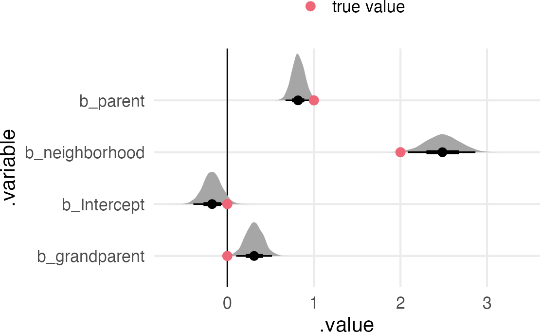
Including the variable haunting the DAG ought to improve things, but in reality that assumes we know what it is, and have some measure of it.

Exorcised model

brm(
  child ~ parent + grandparent + neighborhood,
  data = haunted_sim,
  prior = c(
    prior(normal(0,3), class = b)
  ),
  backend = "cmdstanr",
  cores = 4,
  file = "exorcised1"
)->
  exorcised1_mod

true params

tribble(
  ~.variable, ~.value,
  "b_Intercept", 0,
  "b_grandparent", b_GC,
  "b_parent", b_PC,
  "b_neighborhood", b_N
)->
  true_param

exorcised params

exorcised1_mod |> 
  gather_draws(
    `b_.*`,
    regex = T 
  ) ->
  exorcised1_params

Code

exorcised1_params |> 
  ggplot(
    aes(
      .value,
      .variable
    )
  ) +
    geom_vline(xintercept = 0)+
    stat_halfeye()+
    geom_point(
      data = true_param,
      aes(color = "true value"),
      size = 3
    )+
    scale_color_manual(
      values = ptol_red,
      name = NULL
    )+
    theme(
      legend.position = "top"
    )

I’m not sure why my posterior estimates are so much further off from McElreath’s…