Linear Models: Part 1

Listening

Loading

library(tidyverse)
library(ggdist)
library(here)

source(here("_defaults.R"))

Simulating a Galton Board

“Suppose you and a thousand of your closest friends line up in the halfway line of a soccer field.”

Ok, so the N is 1+1,000 (“you and 1000 of your closest friends”). Apparently a soccer field is 360 feet long, and an average stride length is something like 2.3 feet.

(360/2)/2.3

[1] 78.26087

We can get in 78 steps from the halfway line to the end of the field.

set.seed(500)

expand_grid(
  person = 1:1001,
  step = 1:78
) |> 
  mutate(
    flip = sample(
      c(-1, 1), 
      size = n(), 
      replace = T
    )
  ) |> 
  mutate(
    .by = person,
    position = cumsum(flip)
  ) ->
  galton_board

galton_board |> 
  mutate(
    .by = c(step, position),
    n = n()
  ) ->
  galton_board

galton_board |> 
  ggplot(
    aes(step, position)
  )+
    geom_line(
      aes(group = person, color = n)
    ) +
  scale_x_reverse()+
  khroma::scale_color_bilbao(
      guide = "none"
    )+  
  coord_flip()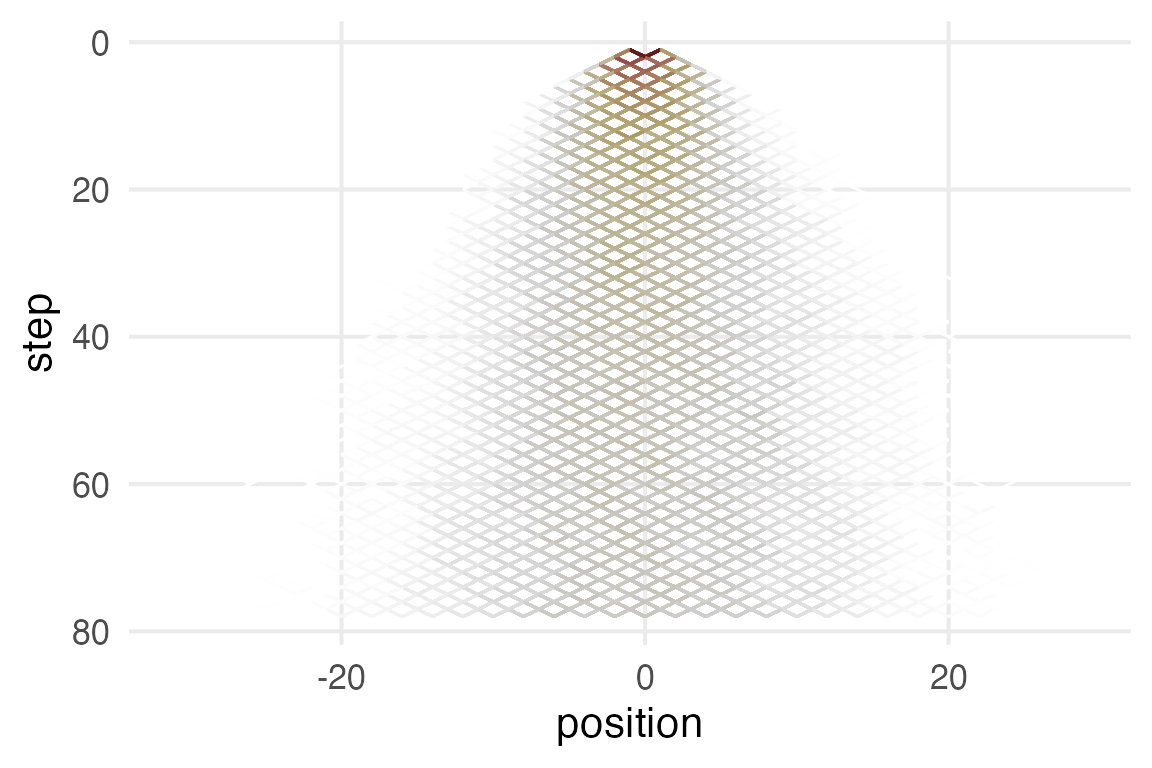

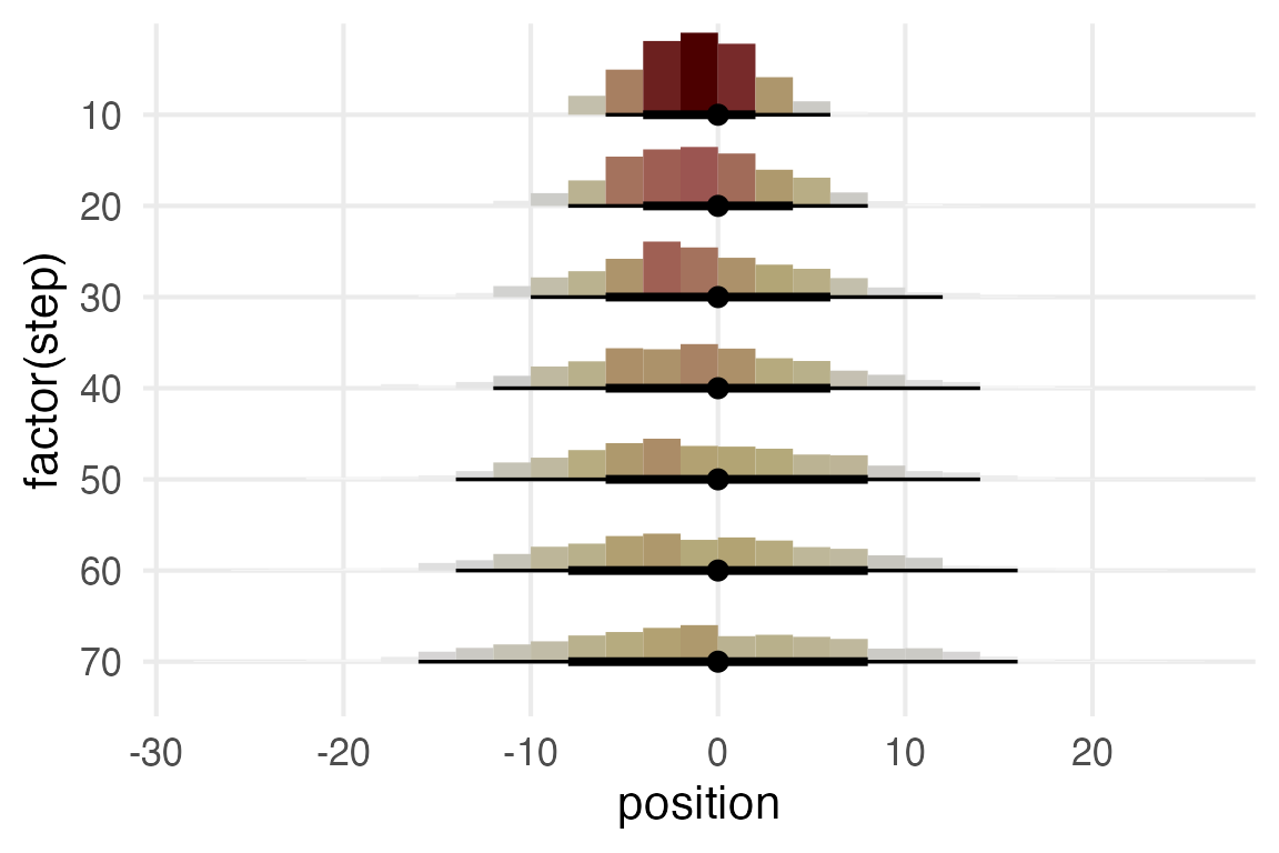
It’s hard to visualize well with the completely overlapping points. I’ll plot histograms for very 10th step.

galton_board |> 
  filter(step %in% seq(10, 70, by = 10)) |> 
  ggplot(aes(position, factor(step)))+
    stat_histinterval(
      breaks = breaks_fixed(width = 2),
      aes(fill = after_stat(pdf))
    )+
    khroma::scale_fill_bilbao(
      guide = "none"
    )+
    scale_y_discrete(
      limits = factor(seq(70, 10, by = -10))
    )

Infinitesimal Galton Board

Same as before, but now instead of flipping a coin for -1 and 1, values are sampled from \(\mathcal{U}(-1,1)\).

expand_grid(
  person = 1:1001,
  step = 1:78
) |> 
  mutate(
    flip = runif(
      n(),
      -1,
      1
    )
  ) |> 
  mutate(
    .by = person,
    position = cumsum(flip)
  ) ->
  inf_galton_board

inf_galton_board |> 
  ggplot(aes(step, position))+
    geom_line(
      aes(group = person),
      alpha = 0.05
    )+
  scale_x_reverse()+
  coord_flip()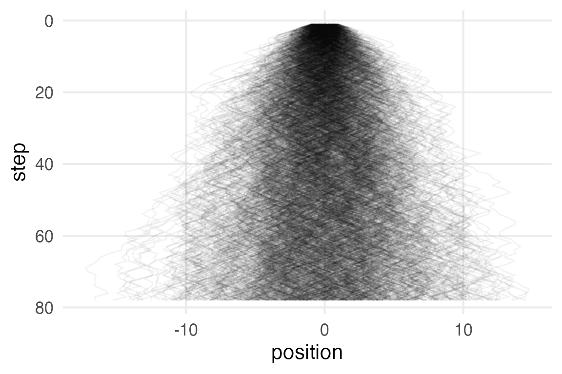

inf_galton_board |> 
  filter(step %in% seq(10, 70, by = 10)) |> 
  ggplot(aes(position, factor(step)))+
    stat_slabinterval(
      aes(fill = after_stat(pdf)), 
      fill_type = "gradient"
    )+
    khroma::scale_fill_bilbao(
      guide = "none"
    )+
    scale_y_discrete(
      limits = factor(seq(70, 10, by = -10))
    )

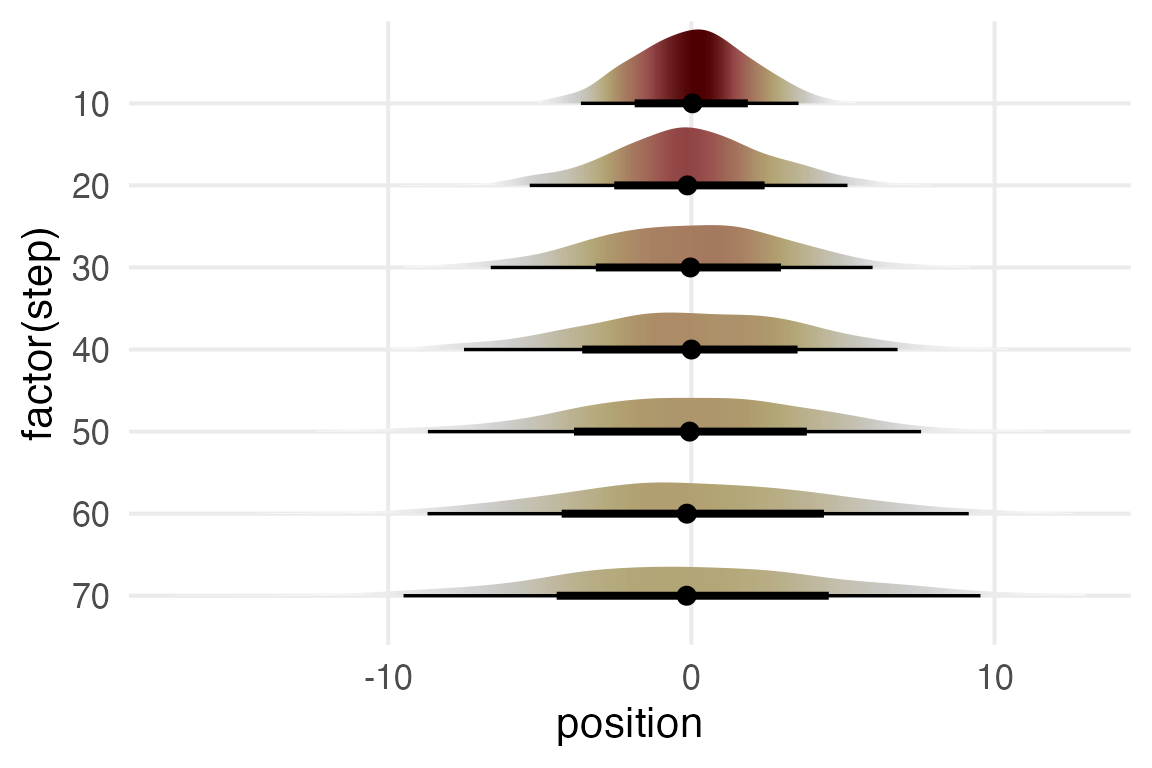
Nice.

I’m not 100% sure how to get a normal density estimate superimposed in that same plot. So I’ll fake it instead.

inf_galton_board |> 
  filter(step %in% seq(10, 70, by = 10)) ->
  ten_steps

ten_steps |> 
  summarise(
    .by = step,
    mean = mean(position),
    sd = sd(position)
  ) |> 
  nest(
    .by = step
  ) |> 
  mutate(
    dist = map(
      data,
      ~tibble(
        position = seq(-20, 20, length = 100),
        dens = dnorm(
          position, 
          mean = .x$mean, 
          sd = .x$sd
        )
      )
    )
  ) |> 
  unnest(dist) |> 
  mutate(
    dens_norm = dens/max(dens)
  )->
  distributions

1

Calculating the distribution parameters for each step grouping.

2

Mapping over the distribution parameters to get density values in a tibble.

3

For plotting over the stat_slab() output, normalizing the density to max out at 1.

ten_steps |> 
  ggplot(aes(position))+
    stat_slabinterval(
      aes(fill = after_stat(pdf)), 
      fill_type = "gradient"
    )+
    geom_line(
      data = distributions,
      aes(y = dens_norm)
    )+
    khroma::scale_fill_bilbao(
      guide = "none"
    )+
    facet_wrap(
      ~step, labeller = label_both
    )+
    theme_no_y()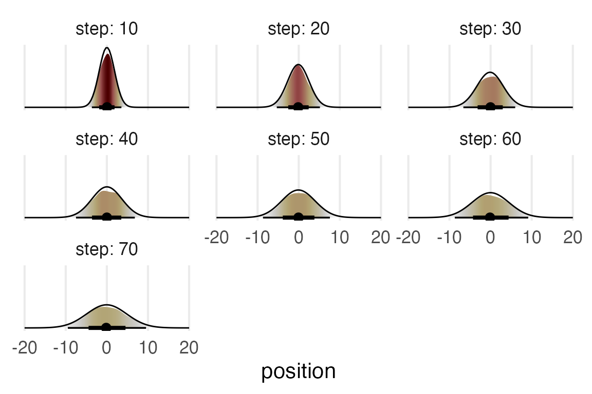

Comparing parameters

For my own interest, I wonder how much discrete sampling from -1, 1 vs the uniform distribution affects the \(\sigma\).

galton_board |> 
  summarise(
    .by = step,
    pos_sd = sd(position)
  ) |> 
  mutate(
    sampling = "discrete"
  ) ->
  galton_sd

inf_galton_board |> 
  summarise(
    .by = step,
    pos_sd = sd(position)
  ) |> 
  mutate(
    sampling = "uniform"
  )->
  inf_galton_sd

bind_rows(
  galton_sd, 
  inf_galton_sd
) |> 
  ggplot(aes(step, pos_sd))+
    geom_line(
      aes(color = sampling),
      linewidth = 1
    )+
    expand_limits(y = 0)+
    labs(
      y = expression(sigma)
    )

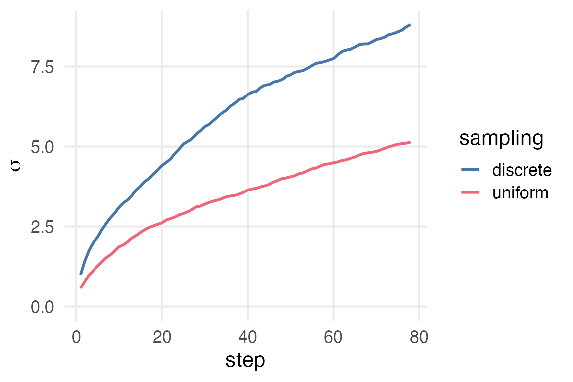
Messing around with a few obvious values of \(x\), in \(\mathcal{U}(-x,x)\), I can’t tell what would approximate the discrete sampling. 2 is too large, and 1.5 is too small. The answer is probably some horror like \(\frac{\pi}{e}\).¹

Model Diagrams

Here’s the model described in the text.

\[ y_i \sim \mathcal{N}(\mu_i, \sigma) \]

\[ \mu_i = \beta x_i \]

\[ \beta \sim \mathcal{N}(0, 10) \]

\[ \sigma \sim \text{Exponential}(1) \]

He also defines a sampling distribution over \(x_1\), but idk if that’s right. Here’s my attempt at converting that into a mermaid diagram.

flowchart RL
  normal1["N(μᵢ, σ)"] -->|"~"| y["yᵢ"]
  beta["β"] --> mult1(["×"])
  x[xᵢ] --> mult1
  mult1 --> mu1[μᵢ]
  mu1 --> normal1
  
  exp1["Exp(1)"] --"~"--> sigma1[σ]
  sigma1 --> normal1
  
  normal2["N(0,10)"] --"~"--> beta

It’s ok. No quite a Kruschke diagram.

Another example.

Let me try to write out the diagram for something like y ~ x + (1|z).

\[ y \sim(\mu_i, \sigma_0) \]

\[ \mu_i = \beta_0 + \beta_1x_i + \gamma_i \]

\[ \beta_0 \sim \mathcal{N}(0,10) \]

\[ \beta_2 \sim \mathcal{N}(0,2) \]

\[ \gamma_i = \Gamma_{z_i} \]

\[ \Gamma_j \sim \mathcal{N}(0,\sigma_1) \]

\[ \sigma_0 \sim \text{Exponential}(1) \]

\[ \sigma_1 \sim \text{Exponential}(1) \]

Geeze, idk. That double subscript feels rough, and I don’t know the convention for describing the random effects.

flowchart TD
  normal1["N(μᵢ, σ₀)"] --"~"--> y[yᵢ]
  beta0["β₀"] --> plus(["+"])
  beta1["β₁"] --> plus
  gamma["γᵢ"] --> plus
  plus --> mu["μᵢ"]
  mu --> normal1
  normal2["N(0,10)"] --"~"--> beta0
  normal3["N(0,2)"] --"~"--> beta1
  Gamma["Γ[zᵢ]"] --> gamma
  normal4["N(0, σ₁)"] --"~"--> Gamma
  exponent0["Exp(1)"] --"~"--> sigma0["σ₀"]
  sigma0 --> normal1
  exponent1["Exp(1)"] --"~"--> sigma1["σ₁"]
  sigma1 --> normal4
  

Yeah, this is too tall. Will have to think about this. The Krushke style diagram is the most compressed version imo.

Footnotes

1. Not literally \(\frac{\pi}{e}\) though, cause that’s too small at 1.156