Statistical Rethinking Workthrough Blog - Multicollinearity & Post-treatment bias

Listening

Setup

Code

library(tidyverse)
library(tidybayes)
library(brms)
library(gt)
library(gtsummary)
library(patchwork)
library(ggblend)
library(ggdensity)
library(ggforce)
library(marginaleffects)
library(dagitty)
library(ggdag)
library(GGally)


source(here::here("_defaults.r"))

set.seed(2023-9-5)

What to (not) do

Here’s what McElreath says about multicollinearity

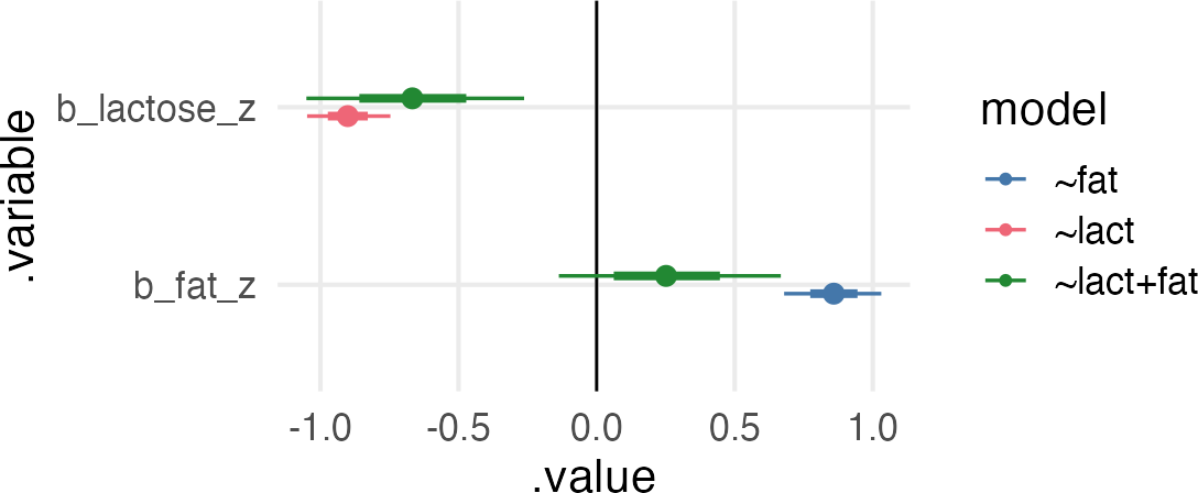
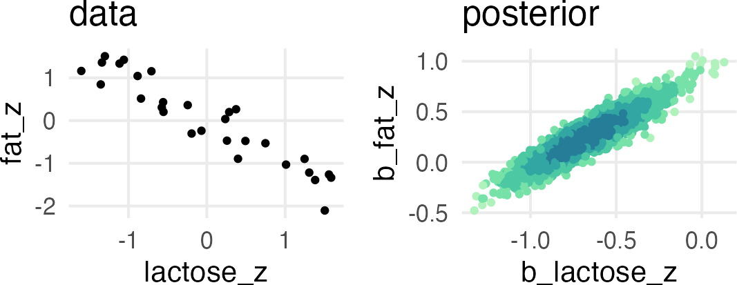
Some fields actually teach students to inspect pairwise correlations before fitting a model, to identify and drop highly correlated predictors. This is a mistake. Pairwise correlations are not the problem. It is the conditional associations—not correlations—that matter. (emphasis added)

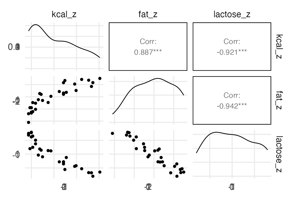
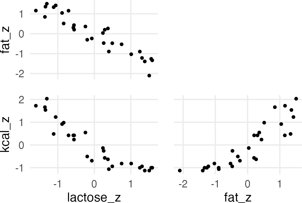
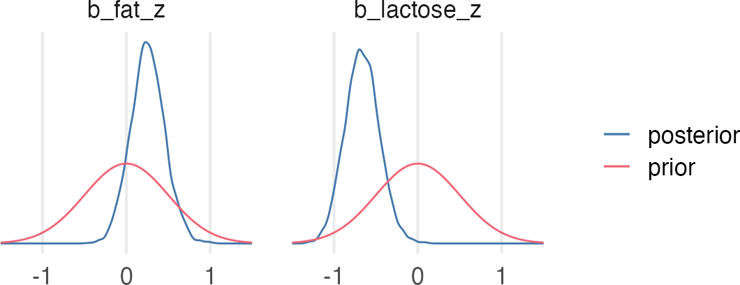
A real multicollinear example

A real multicollinear example involves the percent fat and lactose in primate’s milk when used to predict the kcal.

data(milk, package = "rethinking")

preparing data

milk |> 
  drop_na(
    kcal.per.g, 
    perc.fat, 
    perc.lactose
  ) |> 
  mutate(
    kcal_z = (kcal.per.g-mean(kcal.per.g))/sd(kcal.per.g),
    fat_z = (perc.fat - mean(perc.fat))/sd(perc.fat),
    lactose_z = (perc.lactose - mean(perc.lactose))/sd(perc.lactose)
  )->
  milk_to_mod

I wanted to make a pairs plot with GGally::pairs(), but something is busted with the axes. I’ll have to do it a little by hand.

GGally::pairs() attempt

milk_to_mod |> 
  select(
    ends_with("_z")
  ) |> 
  GGally::ggpairs()

Figure 1: pairs plot of the primate milk data

Code

milk_to_mod |> 
  ggplot(aes(lactose_z, kcal_z)) +
    geom_point()->
  a

milk_to_mod |> 
  ggplot(aes(fat_z, kcal_z))+
    geom_point()+
    theme_blank_y()->
  b

milk_to_mod |> 
  ggplot(aes(lactose_z, fat_z))+
    geom_point()+
    theme_blank_x()->
  c

this_layout <- "
C#
AB
"

a+b+c + plot_layout(design = this_layout)

Ok, now I’ll fit models for

kcal_z ~ lactose_z
kcal_z ~ fat_z
kcal_z ~ lactose_z + fat_z

with the same priors from the book.

model priors

milk_prior <- c(
  prior(normal(0, 0.2), class = Intercept),
  prior(normal(0, 0.5), class = b)
)

lactose model

brm(
  kcal_z ~ lactose_z,
  prior = milk_prior,
  data = milk_to_mod,
  backend = "cmdstanr",
  cores = 4,
  file = "kcal_lact_mod" 
)->
  kcal_lact_mod

fat model

brm(
  kcal_z ~ fat_z,
  prior = milk_prior,
  data = milk_to_mod,
  backend = "cmdstanr",
  cores = 4,
  file = "kcal_fat_mod" 
)->
  kcal_fat_mod

lactose and fat model

brm(
  kcal_z ~ lactose_z + fat_z,
  prior = milk_prior,
  data = milk_to_mod,
  backend = "cmdstanr",
  cores = 4,
  file = "kcal_lact_fat_mod" 
)->
  kcal_lact_fat_mod

Now to compare the estimates

a function

I should really refactor the code chunk below into its own function, but the nonstandard evaluation of gather_draws() is intimidating to me.

getting all betas

list(
  lact = kcal_lact_mod,
  fat = kcal_fat_mod,
  lact_fat = kcal_lact_fat_mod
) |> 
  map(
    ~ .x |> 
      gather_draws(
        `b_.*`,
        regex = T
      )
  ) |> 
  list_rbind(
    names_to = "model"
  ) ->
  all_milk_params

We only want to look at the non-intercept parameters.

dropping intercepts

all_milk_params |> 
  filter(
    str_detect(
      .variable, 
      "Intercept", 
      negate = T
    )
  ) ->
  milk_betas

Code

milk_betas |> 
  mutate(
    model = str_c(
      "~", 
      model
    ) |> 
      str_replace(
        "_",
        "+"
      )
  ) |> 
  ggplot(
    aes(
      .value,
      .variable,
      color = model
    )
  )+
    geom_vline(
      xintercept = 0
    )+
    stat_pointinterval(
      position = position_dodge(width = 0.2)
    )

So, in each separate model, lactose and fat have larger magnitudes than in the model with both.

Lets grab the correlation of the parameters in the full model.

getting parameter correlation.

all_milk_params |> 
  filter(
    model == "lact_fat"
  ) |> 
  pivot_wider(
    names_from = .variable,
    values_from = .value
  ) |> 
  select(
    starts_with("b_")
  ) |> 
  cor() ->
  milk_param_cor

milk_param_cor

            b_Intercept b_lactose_z    b_fat_z
b_Intercept  1.00000000  0.01948817 0.02332534
b_lactose_z  0.01948817  1.00000000 0.92006316
b_fat_z      0.02332534  0.92006316 1.00000000

For fun, let’s make this cleaner for gt

Code

milk_param_cor[
  upper.tri(milk_param_cor, diag = T)
] <- NA

milk_param_cor |> 
  as_tibble(rownames = "param") |> 
  slice(-1) |> 
  select(-b_fat_z) |> 
  gt() |> 
  sub_missing() |> 
  fmt_number() |> 
  cols_label(
    param = ""
  )

	b_Intercept	b_lactose_z
b_lactose_z	0.02	—
b_fat_z	0.02	0.92

Table 1:

Parameter posterior correlation

Notably, the correlation of the b_fat_z and the b_lactose_z parameters ≠ the correlation of the data.

(milk_to_mod |> 
  select(
    lactose_z,
    fat_z
  ) |> 
  cor())[1,2]

[1] -0.9416373

Here’s a visual comparison of the original data versus the posterior estimates for the effect of the variables.

Code

milk_to_mod |> 
  ggplot(
    aes(
      lactose_z,
      fat_z
    )
  )+
    geom_point()+
    labs(
      title = "data"
    )->
  data_cor

all_milk_params |> 
  filter(
    model == "lact_fat"
  ) |> 
  pivot_wider(
    names_from = .variable,
    values_from = .value
  ) |> 
  ggplot(
    aes(
      b_lactose_z, 
      b_fat_z
    )
  )+
    stat_hdr_points()+
    guides(
      color = "none"
    ) +
    labs(title = "posterior")->
  posterior_cor

data_cor + posterior_cor

McElreath says one thing to do is compare the posterior to the prior. Very similar posteriors and priors could indicate identifiability problems.

Code

all_milk_params |> 
  filter(
    model == "lact_fat",
    .variable %in% c("b_lactose_z", "b_fat_z")
  ) |> 
  ggplot(
    aes(
      .value
    )
  )+
  stat_density(
    aes(
      color="posterior"
    ),
    geom = "line"
  )+
  stat_function(
    fun = dnorm,
    args = list(
      mean = 0,
      sd = 0.5
    ),
    aes(
      color = "prior"
    )
  ) +
  facet_wrap(
    ~.variable
  )+
  xlim(
    0.5 * -3,
    0.5 * 3
  )+
  labs(
    color = NULL,
    x = NULL
  )+
  theme_no_y()+
  theme(
    aspect.ratio = 0.8
  )

Post-treatment bias

Making this work is going to involve both wrapping my mind around a post-treatment bias, and figuring out how to set a lognormal prior or family in brms.

The hypothetical situation: You’re testing different antifungal soils on plant growth, and you’re measuring their height, and the presence/absence of fungus. The chronological process is something like:

flowchart LR
  a[measure sprouts]
  b(treat soil)
  a --> b
  c[measure plants]
  d[record fungus]
  b --> c
  b --> d

The causal process might be something like

graph LR
  h0[initial height]
  h1[second height]
  f[fungus]
  t[treatment]
  
  h0 --> h1
  f --> h1
  t --> f

This makes it much clearer now! “Post treatment” meaning “a variable that sits between the treatment and the outcome.”

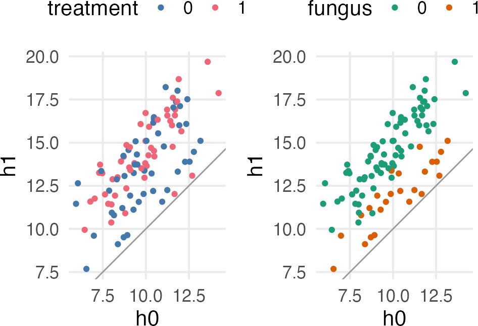
fungus simulation

n = 100
tibble(
  plant_id = 1:n,
  treatment = plant_id %% 2,
  h0 = rnorm(n, 10, 2),
  fungus = rbinom(
    100,
    size = 1,
    prob = 0.5 - treatment * 0.4
  ),
  h1 = h0 + 
    rnorm(
      n, 
      mean = 5 - 3 * fungus
    )
)->
  fungus_sim

Code

fungus_sim |> 
  ggplot(
    aes(
      h0,
      h1,
      color = factor(treatment)
    )
  )+
    geom_point()+
    geom_abline(color = "grey60")+
    labs(
      color = "treatment"
    )+
  theme(
    legend.position = "top",
    aspect.ratio = NULL
  )+
  coord_fixed()->
  fungus1

fungus_sim |> 
  ggplot(
    aes(
      h0,
      h1,
      color = factor(fungus)
    )
  )+
    geom_point()+
    geom_abline(color = "grey60")+
    labs(
      color = "fungus"
    )+
    scale_color_brewer(
      palette = "Dark2"
    )+
  theme(
    legend.position = "top",
    aspect.ratio = NULL
  )+
  coord_fixed()->
  fungus2

fungus1 + fungus2

Figure 6: plant hight, comparing treatment vs fungus effects

Fitting the model

The way the book fits the model is to use a multiplier on h0. To get this to work in brm() , I think I need to use its non-linear modelling capacity.

First, we fit just an across-the-board model, without including treatment or fungus

growth only model

brm(
  bf(
    h1 ~ h0 * p,
    p ~ 1,
    nl = T
  ),
  prior = c(
    prior(lognormal(0, 0.25), coef = Intercept, nlpar = p)
  ),
  data = fungus_sim,
  backend = "cmdstanr",
  file = "fungus1"
)->
  fungus1_mod

getting growth estimate

fungus1_mod |> 
  gather_draws(
    `b_.*`,
    regex = T
  ) -> fungus1_params

Code

fungus1_params |> 
  ggplot(
    aes(
      .value, 
      .variable
    )
  )+
    stat_halfeye()

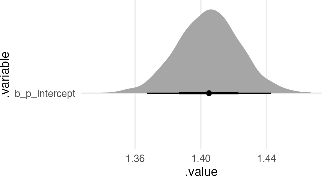
This is, thankfully, very similar to what the posterior from the book was! So maybe I did it right. Let’s grab the maximum likelihood estimate from the simulated data.

data summary stats

fungus_sim |> 
  mutate(
    p = h1/h0
  ) |> 
  reframe(
    stat = c("median", "mean", "logmean"),
    value = c(
      median(p),
      mean(p),
      exp(mean(log(p)))
    )
  ) |> 
  gt() |> 
  fmt_number()

stat	value
median	1.45
mean	1.43
logmean	1.42

Table 2:

Summary stats of the growth data.

Including both predictors

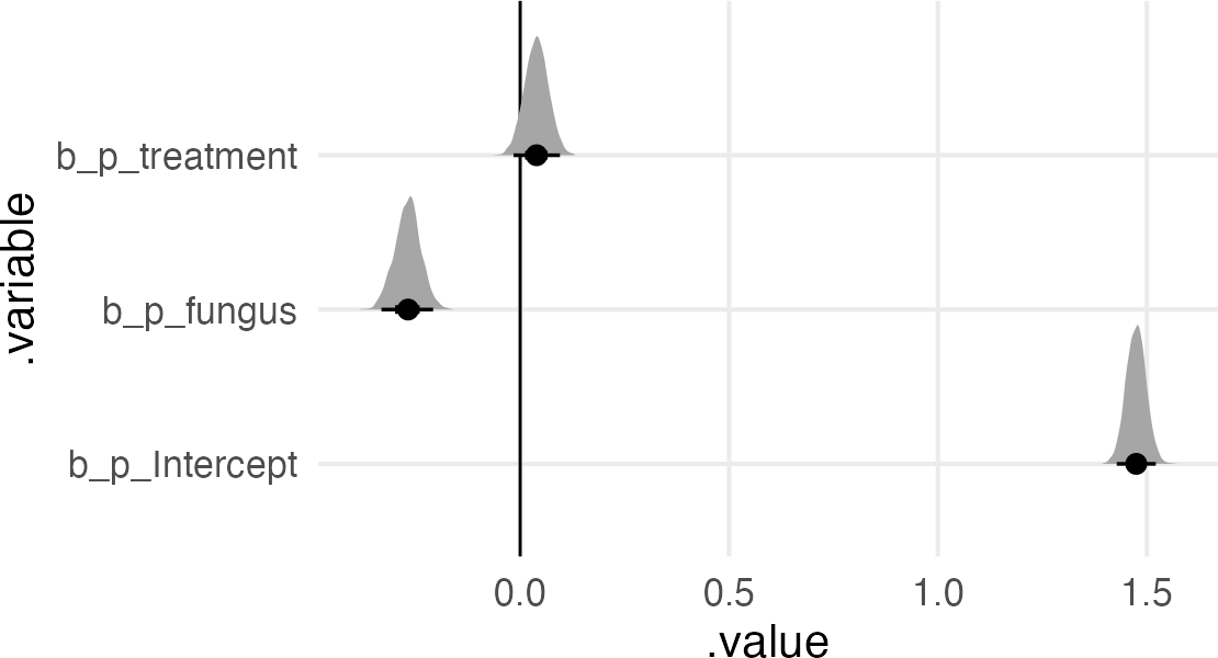
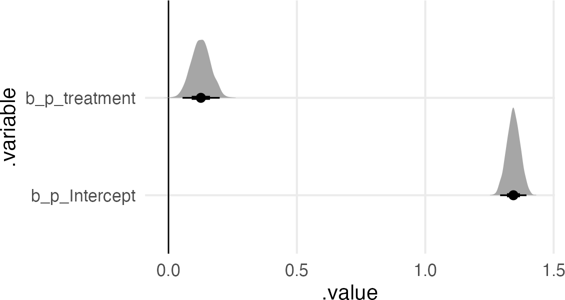
Now we’ll do the “bad” thing and include both predictors. The book keeps the lognormal prior on the intercept of the multiplier, but just a normal prior on the treatment and fungus effects.

fungus + treatment model

brm(
  bf(
    h1 ~ h0 * p,
    p ~ treatment + fungus,
    nl = T
  ),
  prior = c(
    prior(lognormal(0, 0.2), coef = Intercept, nlpar = p),
    prior(normal(0, 0.5), coef = treatment, nlpar = p),
    prior(normal(0, 0.5), coef = fungus, nlpar = p)
  ),
  data = fungus_sim,
  backend = "cmdstanr",
  file = "fungus2"
)->
  fungus2_mod

getting parameters

fungus2_mod |> 
  gather_draws(
    `b_.*`,
    regex = T
  )->
  fungus2_param

Code

fungus2_param |> 
  mutate(
    .variable = .variable |> 
      as.factor() |> 
      fct_relevel(
      "b_p_Intercept",
      after = Inf
    )
  ) |> 
  ggplot(
    aes(
      .value,
      .variable
    )
  )+
    geom_vline(xintercept = 0)+
    stat_halfeye()

Ok, so just like the book

The multiplier intercept got bigger (since it’s the growth for treatment=0, fungus=0).
We’ve got a negative effect of fungus.
We’ve got a weak or 0 effect of treatment.

The non-effect of treatment makes sense, since the effect of treatment is conditional on the effect of the fungus, and the presence/absence of fungus is itself an outcome of the treatment.

But, this doesn’t mean the treatment didn’t work. There are a lot more plants without fungus in the treatment condition than the non-treatment.

treatment by fungus

fungus_sim |> 
  count(
    treatment, fungus
  ) |> 
  pivot_wider(
    names_from = fungus,
    values_from = n
  ) |> 
  gt() |> 
  tab_spanner(
    columns = 2:3,
    label = "fungus"
  )

treatment	fungus
treatment	0	1
0	29	21
1	47	3

Table 3:

Treatment by Fungus

Treatment only

Let’s fit one more model, leaving out fungus.

treatment only model

brm(
  bf(
    h1 ~ h0 * p,
    p ~ treatment,
    nl = T
  ),
  prior = c(
    prior(lognormal(0, 0.2), coef = Intercept, nlpar = p),
    prior(normal(0, 0.5), coef = treatment, nlpar = p)
  ),
  data = fungus_sim,
  backend = "cmdstanr",
  file = "fungus3"
)->
  fungus3_mod

getting treatment only params

fungus3_mod |> 
  gather_draws(
    `b_.*`,
    regex = T
  ) ->
  fungus3_param

Code

fungus3_param |> 
  ggplot(
    aes(
      .value, 
      .variable
    )
  )+
    geom_vline(
      xintercept = 0
    ) +
    stat_halfeye()

Figure 8: Estimates from treatment only model.

Now we get a reliable positive effect of treatment.

Looking at it in a DAG

I’ll use the {ggdag} and {dagitty} packages to build a directed acyclic graph, and then get the “conditional independencies” from it.

The ggdag::dagify() function takes a sequence of formulas that translate back and forth between the dags like so:

# dag
h0 -> h1

# formula
h1 ~ h0

making the dag

# from {ggdag}
dagify(
  h1 ~ h0,
  h1 ~ fungus,
  fungus ~ treatment
)->
  fungus_dag

getting the independencies

impliedConditionalIndependencies(
  fungus_dag
)

fngs _||_ h0
h0 _||_ trtm
h1 _||_ trtm | fngs

So, getting these conditional independence statements to look nice is a whole thing, apparently. There’s a unicode character, ⫫, but in LaTeX the best option is apparently \perp\!\!\!\perp, \(\perp\!\!\!\perp\).

Anyway, the important statement in there is

\[\text{h}1 \perp\!\!\!\perp \text{treatment}~ |~ \text{fungus}\]

This means that if fungus is included, then h1 (our outcome) is independent from treatment, i.e. including the post-treatment effect in the model will make it seem like there’s no effect of the treatment.