Statistical Rethinking Workthrough Blog - Reporting linear model parameters

Listening

Loading

library(tidyverse)
library(tidybayes)
library(gt)
library(gtsummary)

library(brms)
library(marginaleffects)
library(broom.mixed)

source(here::here("_defaults.R"))

Table libraries

library(gtsummary)
library(stargazer)

height_weight_mod <- read_rds(here::here("posts", "2023-06-14_09-reporting", "height_weight_mod.rds"))

The goal

Try to get estimates from this brms model into a table, or some other kind of format, that I like:

height_weight_mod

 Family: gaussian 
  Links: mu = identity; sigma = identity 
Formula: height ~ 1 + weight0 
   Data: height_to_mod (Number of observations: 251) 
  Draws: 4 chains, each with iter = 2000; warmup = 1000; thin = 1;
         total post-warmup draws = 4000

Population-Level Effects: 
          Estimate Est.Error l-95% CI u-95% CI Rhat Bulk_ESS Tail_ESS
Intercept   154.59      0.32   153.93   155.22 1.00     4061     2653
weight0       0.91      0.05     0.81     1.01 1.00     3991     2705

Family Specific Parameters: 
      Estimate Est.Error l-95% CI u-95% CI Rhat Bulk_ESS Tail_ESS
sigma     5.16      0.24     4.72     5.64 1.00     4328     3175

Draws were sampled using sampling(NUTS). For each parameter, Bulk_ESS
and Tail_ESS are effective sample size measures, and Rhat is the potential
scale reduction factor on split chains (at convergence, Rhat = 1).

Off-the-shelf table methods

{gtsummary} has a tbl_regression() function.

height_weight_mod |> 
  gtsummary::tbl_regression(
    intercept = T
  )

Characteristic	Beta	95% CI¹
(Intercept)	155	154, 155
weight0	0.91	0.81, 1.0
¹ CI = Credible Interval

It’s ok.

I know {stargazer} is a package people use for reporting models.

data(penguins, package = "palmerpenguins")

penguin_mod <- lm(bill_length_mm ~ body_mass_g + species, penguins)

stargazer::stargazer(penguin_mod, type = "html")


	Dependent variable:

	bill_length_mm

body_mass_g	0.004^***
	(0.0003)

speciesChinstrap	9.921^***
	(0.351)

speciesGentoo	3.558^***
	(0.486)

Constant	24.919^***
	(1.063)


Observations	342
R²	0.808
Adjusted R²	0.806
Residual Std. Error	2.403 (df = 338)
F Statistic	474.006^*** (df = 3; 338)

Note:	p<0.1; p<0.05; p<0.01

To be quite honest, I’m not a big fan of this giant table of everything & asterisks, and it looks like it’s not implemented for brms models anyway.

stargazer::stargazer(height_weight_mod)


% Error: Unrecognized object type.

Oh well.

Graphical summary methods

There’s a few challenges for visualizing this particular model given that the intercept is on such a different scale from the rest of the parameters.

mcmc_plot(height_weight_mod)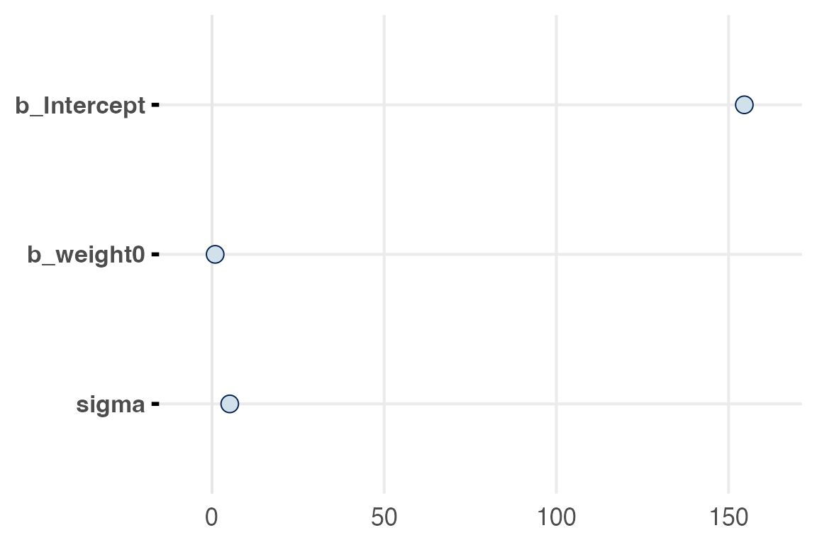

height_weight_mod |> 
  gather_draws(
    `b_.*`,
    sigma,
    regex = TRUE
  ) |> 
  ggplot(aes(.value))+
    stat_slabinterval(
      normalize = "panels",
      point_interval = "mean_hdi"
    )+
    facet_wrap(~.variable, scales = "free", ncol = 1)+
    theme_no_y()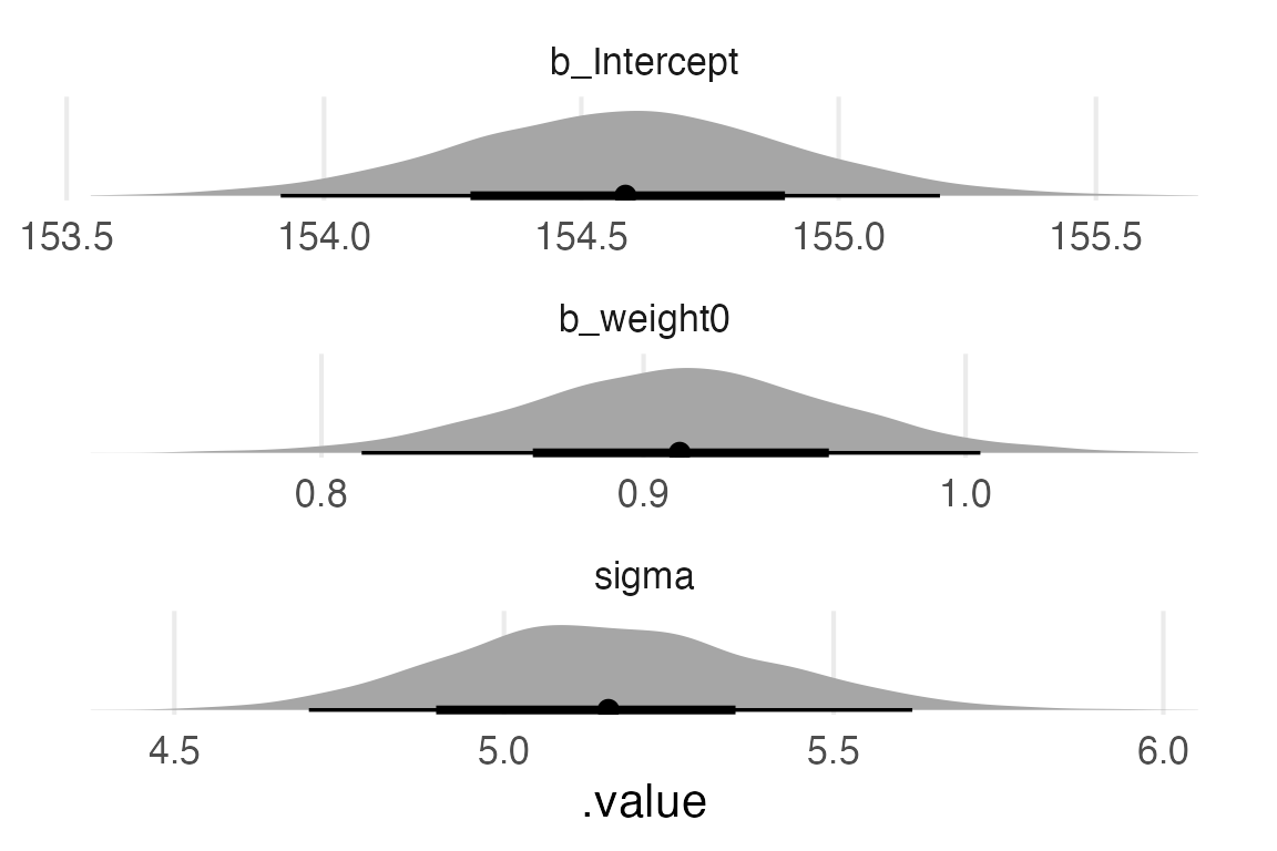

Custom table

I want a custom {gt} table that captures the distributional nature of the posteriors. That’ll involve calculating things like the credible intervals “by-hand” (really, using tidybayes::mean_hdci() and doing some reshaping before the monster {gt} code.

Getting parameter draws

I’ll grab the parameter draws with gather_draws()

height_weight_mod |> 
  gather_draws(
    `b_.*`,
    sigma,
    regex = T 
  ) -> parameter_draws

Getting the parameter summaries

I’ll get the posterior mean and 95% & 50% hdci right now, which results in a long table.

parameter_draws |> 
  group_by(.variable) |> 
  mean_hdci(.value, .width = c(0.95, 0.5)) ->
  initial_table_long

initial_table_long

# A tibble: 6 × 7
  .variable    .value  .lower  .upper .width .point .interval
  <chr>         <dbl>   <dbl>   <dbl>  <dbl> <chr>  <chr>    
1 b_Intercept 155.    154.    155.      0.95 mean   hdci     
2 b_weight0     0.911   0.812   1.00    0.95 mean   hdci     
3 sigma         5.16    4.70    5.62    0.95 mean   hdci     
4 b_Intercept 155.    154.    155.      0.5  mean   hdci     
5 b_weight0     0.911   0.881   0.944   0.5  mean   hdci     
6 sigma         5.16    4.98    5.29    0.5  mean   hdci

Long to wide

What I have right now is a table like

| .variable | .lower | .upper | .width |
| intercept | ...... | ...... |   0.5  |
| intercept | ...... | ...... |   0.95 |

What for my final table will be something like

| .variable | lower_95 | lower_50 | upper_50 | upper_95 |
| intercept | ........ | ........ | ........ | ........ |

So, getting from here to there will involve some pivoting

initial_table_long |> 
  pivot_longer(
    .lower:.upper,
    names_to = "side",
    values_to = "side_value"
  ) |> 
  unite(
    col = "side",
    c(side, .width)
  ) |> 
  pivot_wider(
    names_from = side,
    values_from = side_value
  ) |> 
  relocate(
    ends_with("_0.5"),
    .after = .lower_0.95
  ) |> 
  select(-.point, -.interval) ->
  initial_table_wide

initial_table_wide

# A tibble: 3 × 6
  .variable    .value .lower_0.95 .lower_0.5 .upper_0.5 .upper_0.95
  <chr>         <dbl>       <dbl>      <dbl>      <dbl>       <dbl>
1 b_Intercept 155.        154.       154.       155.         155.  
2 b_weight0     0.911       0.812      0.881      0.944        1.00
3 sigma         5.16        4.70       4.98       5.29         5.62

Posterior sd

I also want to grab the posterior standard deviation, maybe just cause I’m old fashioned, I’ll have to calculate that back with the original posterior draws and then join it onto the table I’m making.

parameter_draws |> 
  group_by(.variable) |> 
  summarise(
    posterior_sd = sd(.value)
  ) ->
  posterior_sd

posterior_sd

# A tibble: 3 × 2
  .variable   posterior_sd
  <chr>              <dbl>
1 b_Intercept       0.324 
2 b_weight0         0.0488
3 sigma             0.237

initial_table_wide |> 
  left_join(posterior_sd) |> 
  relocate(
    posterior_sd,
    .after = .value
  ) ->
  final_report_table

final_report_table

# A tibble: 3 × 7
  .variable    .value posterior_sd .lower_0.95 .lower_0.5 .upper_0.5 .upper_0.95
  <chr>         <dbl>        <dbl>       <dbl>      <dbl>      <dbl>       <dbl>
1 b_Intercept 155.          0.324      154.       154.       155.         155.  
2 b_weight0     0.911       0.0488       0.812      0.881      0.944        1.00
3 sigma         5.16        0.237        4.70       4.98       5.29         5.62

The `{gt}` code

One last bit of clean up will be to the variable names, and creating a group column so I can separate the intercept and weight parameters from the variance parameter.

final_report_table |> 
  ungroup() |> 
  mutate(
    group = case_when(
      str_detect(.variable, "b_") ~ "β",
      .default = "variance"
    ),
    .variable = str_remove(.variable, "b_")
  ) |> 
  group_by(group) ->
  for_gt

for_gt |> 
  gt()->
  gt_interim_01

gt_interim_01

.variable	.value	posterior_sd	.lower_0.95	.lower_0.5	.upper_0.5	.upper_0.95
β
Intercept	154.5857634	0.32423855	153.9159103	154.3976375	154.8290184	155.196791
weight0	0.9112191	0.04884185	0.8124778	0.8805526	0.9442994	1.004583
variance
sigma	5.1583113	0.23732630	4.7040727	4.9795864	5.2942085	5.619339

That’s too many decimal places.

gt_interim_01 |> 
  fmt_number(decimals = 2) ->
  gt_interim_02

gt_interim_02

.variable	.value	posterior_sd	.lower_0.95	.lower_0.5	.upper_0.5	.upper_0.95
β
Intercept	154.59	0.32	153.92	154.40	154.83	155.20
weight0	0.91	0.05	0.81	0.88	0.94	1.00
variance
sigma	5.16	0.24	4.70	4.98	5.29	5.62

Next, I’ll add spanners for the credible intervals, and point estimates.

gt_interim_02 |> 
   tab_spanner(
    label = "50% HDI",
    columns = .lower_0.5:.upper_0.5
  ) |> 
  tab_spanner(
    label = "95% HDI",
    columns = .lower_0.95:.upper_0.95
  ) |> 
  tab_spanner(
    label = "posterior estimates",
    columns = c(.value, posterior_sd)
  ) ->
  gt_interim_03

gt_interim_03

			95% HDI
.variable	posterior estimates		.lower_0.95	50% HDI		.upper_0.95
.variable	.value	posterior_sd	.lower_0.95	.lower_0.5	.upper_0.5	.upper_0.95
β
Intercept	154.59	0.32	153.92	154.40	154.83	155.20
weight0	0.91	0.05	0.81	0.88	0.94	1.00
variance
sigma	5.16	0.24	4.70	4.98	5.29	5.62

With the spanners in place, we can adjust the actual column labels.

gt_interim_03 |> 
   cols_label(
    .variable = md("**parameter**"),
    .value = md("**mean**"),
    posterior_sd = md("**sd**"),
    .lower_0.95:.upper_0.95 ~ ""
  )->
  gt_interim_04

gt_interim_04

			95% HDI
parameter	posterior estimates			50% HDI
parameter	mean	sd
β
Intercept	154.59	0.32	153.92	154.40	154.83	155.20
weight0	0.91	0.05	0.81	0.88	0.94	1.00
variance
sigma	5.16	0.24	4.70	4.98	5.29	5.62

Now, to add some visual clarity to the credible intervals. I’ll fill with ptol_blue, (hex code #4477aa).

gt_interim_04 |> 
  tab_style(
    style = cell_fill(
      color = ptol_blue, 
      alpha = 0.5
      ),
    locations = cells_body(
      columns = ends_with("_0.5")
    )
   ) |> 
  tab_style(
    style = cell_fill(
      color = ptol_blue, 
      alpha = 0.2
      ),
    locations = cells_body(
      columns = ends_with("_0.95")
    )
   )->
  gt_interim_05

gt_interim_05

			95% HDI
parameter	posterior estimates			50% HDI
parameter	mean	sd
β
Intercept	154.59	0.32	153.92	154.40	154.83	155.20
weight0	0.91	0.05	0.81	0.88	0.94	1.00
variance
sigma	5.16	0.24	4.70	4.98	5.29	5.62

For me, the group labels are too visually similar to the names of parameter values, so I’ll style those too.

gt_interim_05 |> 
  tab_style(
    style = cell_text(
      style = "italic", 
      size = "small"
    ),
    locations = cells_row_groups()
  ) ->
  gt_interim_06

gt_interim_06

			95% HDI
parameter	posterior estimates			50% HDI
parameter	mean	sd
β
Intercept	154.59	0.32	153.92	154.40	154.83	155.20
weight0	0.91	0.05	0.81	0.88	0.94	1.00
variance
sigma	5.16	0.24	4.70	4.98	5.29	5.62

Final steps, just adding some header and footer information

gt_interim_06 |> 
  tab_header(
    title = "height ~ weight0"
  ) |> 
  tab_source_note(
    source_note = md("**priors:**<br>intercept &tilde; N(178, 20)<br>β &tilde; N(0,10)<br>σ &tilde; U(0,50)")
  )->
  final_gt_table

final_gt_table

			95% HDI
height ~ weight0
parameter	posterior estimates			50% HDI
parameter	mean	sd
β
Intercept	154.59	0.32	153.92	154.40	154.83	155.20
weight0	0.91	0.05	0.81	0.88	0.94	1.00
variance
sigma	5.16	0.24	4.70	4.98	5.29	5.62
priors: intercept ˜ N(178, 20) β ˜ N(0,10) σ ˜ U(0,50)

I’ll just save this table as a png to be the post image.

gtsave(final_gt_table, filename = "final_gt_table.png")

Was it worth it?

That was a lot of fuss, but a lot of those steps I might roll into my own functions for an actual paper.