Statistical Rethinking Workthrough Blog

Listening

Setup

Code

library(tidyverse)
library(tidybayes)
library(brms)
library(gt)
library(gtsummary)
library(patchwork)
library(ggblend)
library(ggforce)
library(marginaleffects)
library(modelsummary)
library(dagitty)
library(ggdag)

source(here::here("_defaults.r"))

set.seed(2023-9-1)

Newsworthiness & Trustworthiness

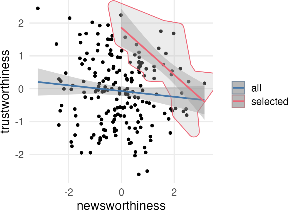
The first example in the book is about Berkson’s Paradox, which I believe is a kind of selection bias. The question is “Why do so many research results that are newsworthy seem unreliable?” The idea being that funding (or whatever, maybe “editorial decisions to publish a paper”) is based jointly on its trustworthiness and its newsworthiness.

tibble(
  trustworthiness = rnorm(200),
  newsworthiness = rnorm(200),
  score = trustworthiness + newsworthiness,
  score_percentile = ecdf(score)(score)
) ->
  research

Code

research |> 
  filter(
    score_percentile >= 0.9
  )->
  selected

research |> 
  ggplot(
    aes(
      newsworthiness,
      trustworthiness
    )
  )+
    geom_point()+
    geom_mark_hull(
      aes(
        filter = score_percentile >= 0.9,
        color = "selected"
      ),
      fill = "grey"
    )+
    stat_smooth(
      aes(
        color = "all"
      ),
      method = lm
    )+
    stat_smooth(
      data = selected,
      aes(
        color = "selected"
      ),
      method = lm
    )+
    coord_fixed()+
    theme(
      aspect.ratio = 1
    )+
    labs(
      color = NULL
    )

Figure 1: The selection effect on the (non)correation between newsworthiness and trustworthiness

Multicollinearity

In fact, there is nothing wrong with multicollinearity. The model will work fine for prediction. You will just be frustrated trying to understand it.

When I was starting to get into advanced statistical modelling during my PhD (some time around 2010?) everyone suddenly learned about multicollinearity and got freaked out about it, so this was genuinely new info to me. See also Vanhove (2021), Collinearity isn’t a disease that needs curing.

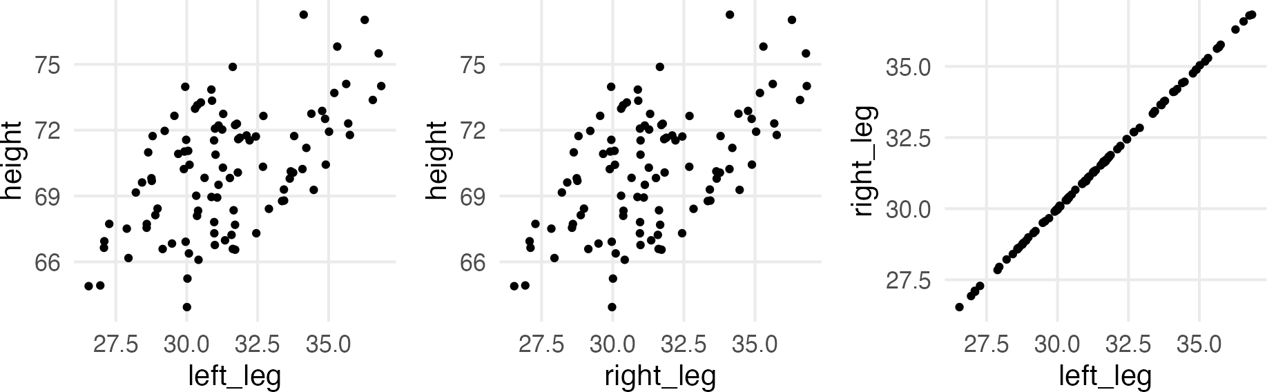
The illustration from the book was about the relationship between total body height and leg length.

leg-heigh simulation

tibble(
  n = 100,
  # height in inches
  height = rnorm(n, mean = 70, sd = 3),
  # legs as a proportion of height
  leg_prop = runif(n, 0.4, 0.5),
  left_leg = height * leg_prop,
  right_leg = left_leg + 
    rnorm(n, sd = 0.02)
)->
  height_legs

The simulated right leg length is going to be, max, ±0.06 (¹⁄₁₆^th inch) the left leg.

Code

height_legs |> 
  ggplot(aes(left_leg, height))+
    geom_point()+
    theme(aspect.ratio = 1)->
  lh

height_legs |> 
  ggplot(aes(right_leg, height))+
    geom_point()+
    theme(aspect.ratio = 1)->
  rh

height_legs |> 
  ggplot(aes(left_leg, right_leg))+
    geom_point()+
    theme(aspect.ratio = 1)->
  lr

lh + rh +lr

A model with only left or right leg is going to be fine.

left leg model

brm(
  height ~ left_leg,
  data = height_legs,
  prior = c(
    prior(normal(70, 100), class = Intercept),
    prior(normal(0, 10), class = b)
  ),
  backend = "cmdstanr",
  file = "height_left"
)->
  height_left_mod

The right leg model:

right leg model

brm(
  height ~ right_leg,
  data = height_legs,
  prior = c(
    prior(normal(70, 100), class = Intercept),
    prior(normal(0, 10), class = b)
  ),
  backend = "cmdstanr",
  file = "height_right"
)->
  height_right_mod

I’m going to get a little fancy to get the parameter estimates from both models all at once.

getting parameter estimates

list(
  left = height_left_mod,
  right = height_right_mod
) |> 
  map(
    ~ gather_draws(
      .x, 
      `.*_leg`,
      regex = T
    )
  ) |> 
  list_rbind(
    names_to = "model"
  )->
  rl_params

Code

rl_params |> 
  ggplot(
    aes(
      .value, 
      .variable,
    )
  )+
    stat_halfeye(
      aes(
        fill = model
      )
    )+
  expand_limits(
    x = 0
  )+
  ylim(
    "b_right_leg",
    "b_left_leg"
  )

But if we include both left and right leg, the estimate of each one’s parameter gets weird.

both leg model

brm(
  height ~ left_leg + right_leg,
  data = height_legs,
  prior = c(
    prior(normal(70, 100), class = Intercept),
    prior(normal(0, 10), class = b)
  ),
  backend = "cmdstanr",
  file = "height_both"
)->
  height_both_mod

getting parameter estimates

list(
  left = height_left_mod,
  right = height_right_mod,
  both = height_both_mod
) |> 
  map(
    ~ gather_draws(
      .x, 
      `.*_leg`,
      regex = T
    )
  ) |> 
  list_rbind(
    names_to = "model"
  )->
  all_params

Code

all_params |> 
  mutate(
    model = model |>  
      fct_relevel("both", after = Inf)
  ) |> 
  ggplot(
    aes(
      .value, 
      .variable,
    )
  )+
    stat_pointinterval(
      aes(
        color = model
      ),
      position = "dodge"
    )+
  expand_limits(
    x = 0
  )+
  ylim(
    "b_right_leg",
    "b_left_leg"
  )

This was the kind of outcome that I was taught to do things like residualize, but McElreath says that while the model we tried to write out was:

\[ \text{height} = \text{Intercept} + \beta_1\text{left} + \beta_2\text{right} \]

because the right leg and the left leg are basically the same, we have something more like

\[ \text{height} = \text{Intercept} + (\beta_1 + \beta_2)\text{leg} \]

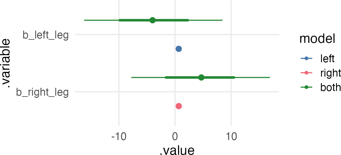
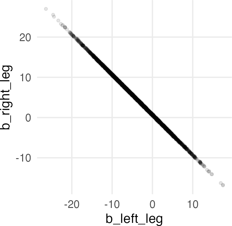
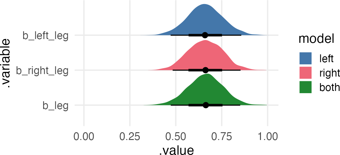
And because there’s nothing else in the model to specify what the value of \(\beta_1\) and \(\beta_2\) are, they’re all over the place. But crucially, they ought to add up to a similar value to what we got for just left_leg and right_leg in the first two models. They also should be negatively correlated, so when one is large and positive, the other should be large and negative, so they cancel out to around the values we got before.

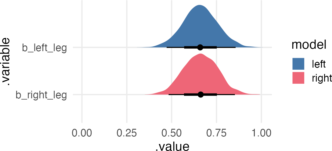
the multicollinear estimates

height_both_mod |> 
  spread_draws(
    `.*_leg`,
    regex = T
  )->
  leg_ests

Code

leg_ests |> 
  ggplot(
    aes(
      b_left_leg,
      b_right_leg
    )
  )+
    geom_point(
      alpha = 0.1
    )+
    coord_fixed()+
    theme(
      aspect.ratio = 1
    )

We can add each parameter together and compare it to the original two models.

adding together multicollinear estimates

leg_ests |> 
  mutate(
    .variable = "b_leg",
    .value = b_left_leg + b_right_leg,
    model = "both"
  ) |> 
  bind_rows(
    rl_params
  ) |> 
  mutate(
    model = fct_relevel(
      model,
      "both",
      after = Inf
    )
  )->
  rl_comp

Code

rl_comp |> 
  ggplot(
    aes(
      .value,
      .variable
    )
  )+
    stat_halfeye(
      aes(
        fill = model
      )
    ) +
  expand_limits(
    x = 0
  ) +
  ylim(
    "b_leg",
    "b_right_leg",
    "b_left_leg"
  )

“The model will work fine for prediction.”

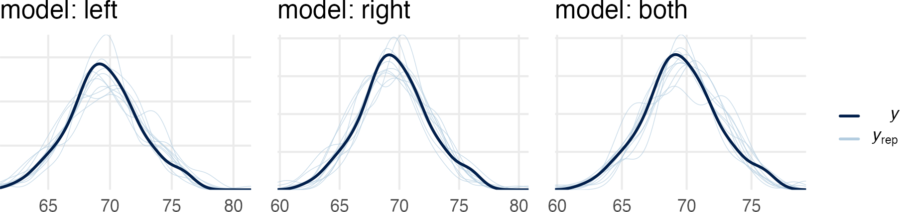
Just to hammer home the point that the predictive value of the multicollinear model, we can compare its posterior predictive checks to the left and right leg models.

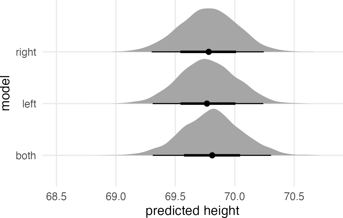
posterior predictive checks

pp_check(height_left_mod)+
  labs(title = "model: left")->
  left_pp

pp_check(height_right_mod)+
  labs(title = "model: right") ->
  right_pp

pp_check(height_both_mod)+
  labs(title = "model: both") ->
  both_pp

left_pp + right_pp + both_pp + plot_layout(guides = "collect")

We can also compare their predictions for new leg length.

getting predicted values

tibble(
  left_leg = 32,
  right_leg = left_leg+0.01
)->
  newleg

list(
  left = height_left_mod,
  right = height_right_mod,
  both = height_both_mod
) |> 
  map(
    ~ predictions(
      .x, 
      newdata = newleg
    ) |> 
      posterior_draws()
  ) |> 
  list_rbind(
    names_to = "model"
  )->
  all_pred

Code

all_pred |> 
  ggplot(
    aes(
      draw,
      model
    )
  )+
    labs(
      x = "predicted height"
    )+
    stat_halfeye()

So what to do?

The upshot of McElreath’s recommendation for what to do about all this multicollinearity is “have a bad time.” There’s no generic answer. Maybe there’s an acceptable way to specify the model depending on the DAG, but also maybe some questions aren’t well put, like “what are the individual contribution of the left leg and the right leg to total height?”

References

Vanhove, Jan. 2021. “Collinearity Isn’t a Disease That Needs Curing.” Meta-Psychology 5 (April). https://doi.org/10.15626/MP.2021.2548.