Introducing tidynorm

The upshot

The tidynorm package has convenience functions for normalizing

Point measurements

Formant Tracks

DCT coefficients

As well as generic functions to implement your own normalization method.

You can install tidynorm in your preferred way from CRAN.

install.packages("tidynorm")

Loading Packages

library(tidynorm)
library(tidyverse)
library(scales)
library(ggtext)
library(gt)
source(here::here("_defaults.R"))

What is speaker vowel normalization?

Imagine a very tall person from London speaking to you. You can probably imagine what their accent sounds like. Now imagine a very short person speaking to you in the same accent. In reality, if you heard these two people speaking in what you perceive to be identical accents, the acoustics of their speech will be different due to their (likely) different vocal tract lengths (VTL).

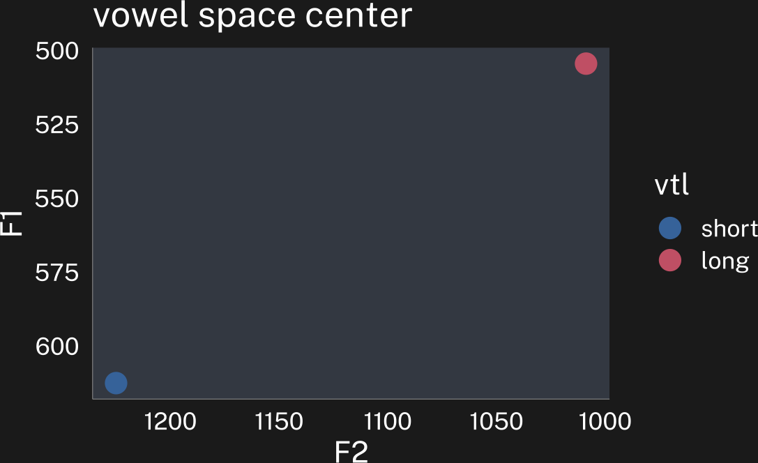
Using some rough heuristics and assumptions, the overall vowel spaces of these two speakers might look something like this:

guestimates functions

vtl_2_formant <- function(vtl, f = 1){
  dF = 34300/(2*vtl)
  dF * (f * 0.5)
}

vowel_polygon <- function(F1, F2){
  tibble(
    F1 = c(
      F1 * 0.6,
      F1 * 1.45,
      F1 * 0.6
      ),
    F2 = c(
      F2 * 1.5,
      F2,
      F2 * 0.52
    )
  )
}

vowel-space-plot

tibble(
  vtl = seq(14, 17, length = 2)
) |> 
  mutate(
    F1 = vtl_2_formant(vtl, 1),
    F2 = vtl_2_formant(vtl, 2),
    F3 = vtl_2_formant(vtl, 3)
  ) |>  mutate(
    vtl = factor(vtl, labels = c("short", "long"))
  ) ->
  speaker_formants

speaker_formants |> 
  reframe(
    .by = vtl,
    vowel_polygon(F1, F2)
  ) |> 
  ggplot(
    aes(F2, F1)
  ) +
  geom_polygon(
    aes(group = vtl, fill = vtl, color = vtl),
    linewidth = 1,
    alpha = 0.6
  ) +
  scale_y_reverse() +
  scale_x_reverse() +
  labs(fill = "VTL", color = "VTL") +
  coord_fixed() -> p

p
p+theme_dark()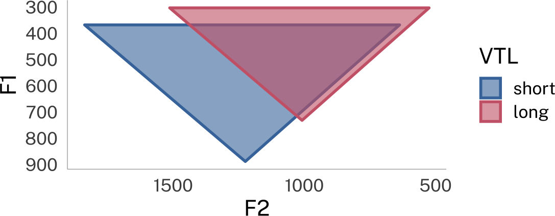

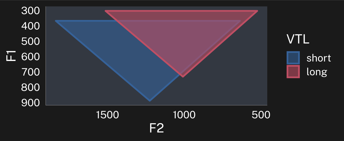
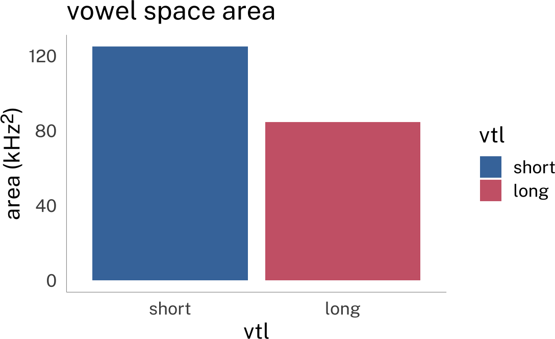
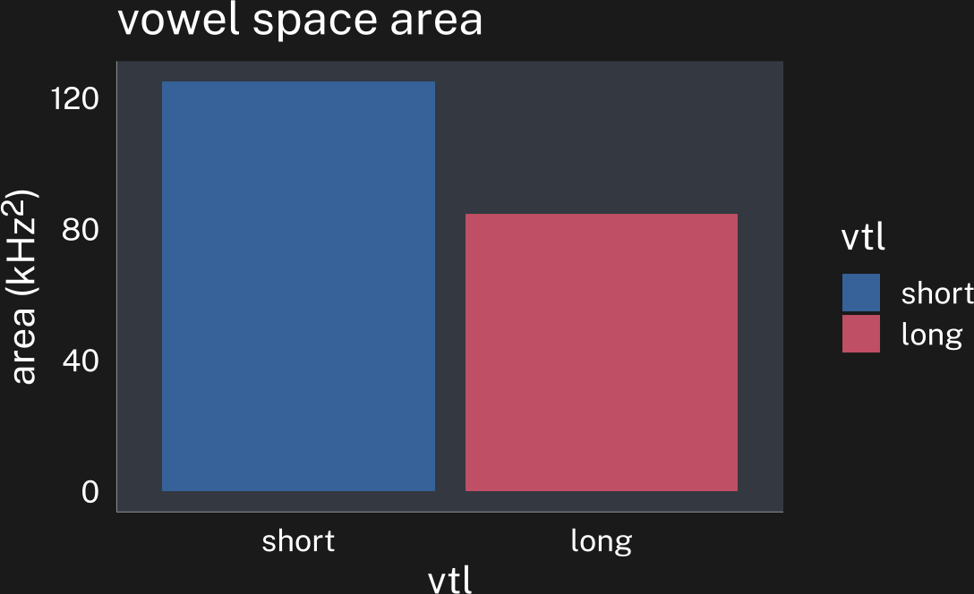
These speakers’ overall vowel spaces have different center points, and cover different areas.

plotting code

speaker_formants |> 
  ggplot(
    aes(F2, F1)
  ) +
  geom_point(
    aes(color = vtl),
    size = 5
  ) +
  scale_y_reverse() +
  scale_x_reverse() +
  labs(title = "vowel space center") -> center_p

speaker_formants |> 
  reframe(
    .by = vtl,
    vowel_polygon(F1, F2)
  ) |> 
  summarise(
    .by = vtl,
    b = diff(range(F1)),
    h = diff(range(F2))
  ) |> 
  mutate(
    a = (b/100 * h/100)*2
  ) |> 
  ggplot(
    aes(
      vtl, a
    )
  )+
  geom_col(aes(fill = vtl)) +
  labs(
    y = "area (kHz<sup>2</sup>)",
    title = "vowel space area"
  )+
  theme(
    axis.title.y = element_markdown()
  ) ->
  area_plot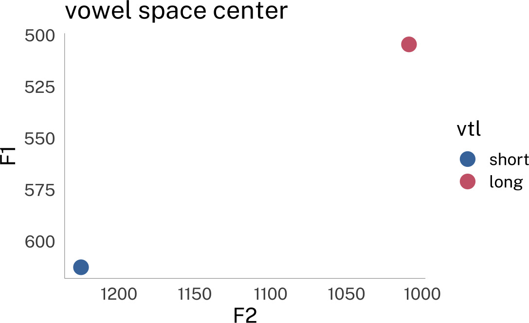

The goal of any speaker vowel normalization method is to try to line up speakers’ vowel spaces so that speaker A’s highest, frontest vowels are lined up with speaker B’s, so that speaker A’s lowest, backest vowels are lined up with speaker B’s, etc. Once we have their vowel spaces aligned in a such way that we know similarities between them are matched, we can start investigating any differences.

Vowel Space ≠ Pitch

One really important thing to keep in mind is that vowel space differences due to different vocal tract lengths are not the same as differences in speakers’ pitch. Differences in speakers’ pitch are caused by differences in how their vocal folds vibrate. You can have two speakers’ with the same exact pitch, but very different vocal tract lengths (& vowel spaces), and vice versa.

Normalization methods

All normalization methods involve some kind of shift in the location of a speaker’s vowel space by some value \(L\), scaling the size of a speaker’s vowel space by some value \(S\), or both.

\[ F' = \frac{F-L}{S} \]

They way normalization methods mainly differ is in terms of

Transformations applied to the original formant values before calculating \(L\) and \(S\) (e.g. log, bark).
The exact functions used to calculate \(L\) and \(S\) (e.g. mean, standard deviation)
The scope over which \(L\) and \(S\) are calculated (e.g. across all formants at once, or one formant at a time).

For example, the logic behind Nearey normalization (Nearey 1978) is that after log transforming vowel spaces, they should really only differ in terms of the location of the centers, not in terms of their area.

plotting code

speaker_formants |> 
  reframe(
    .by = vtl,
    vowel_polygon(F1, F2)
  ) |> 
  mutate(across(F1:F2, log)) |> 
  ggplot(
    aes(F2, F1)
  ) +
  geom_polygon(
    aes(
      group = vtl, 
      fill = vtl, 
      color = vtl
      ),
    alpha = 0.6,
    linewidth = 1
  ) +
  scale_y_reverse("log(F1)") +
  scale_x_reverse("log(F2)") +
  coord_fixed() -> p

p
p+theme_dark()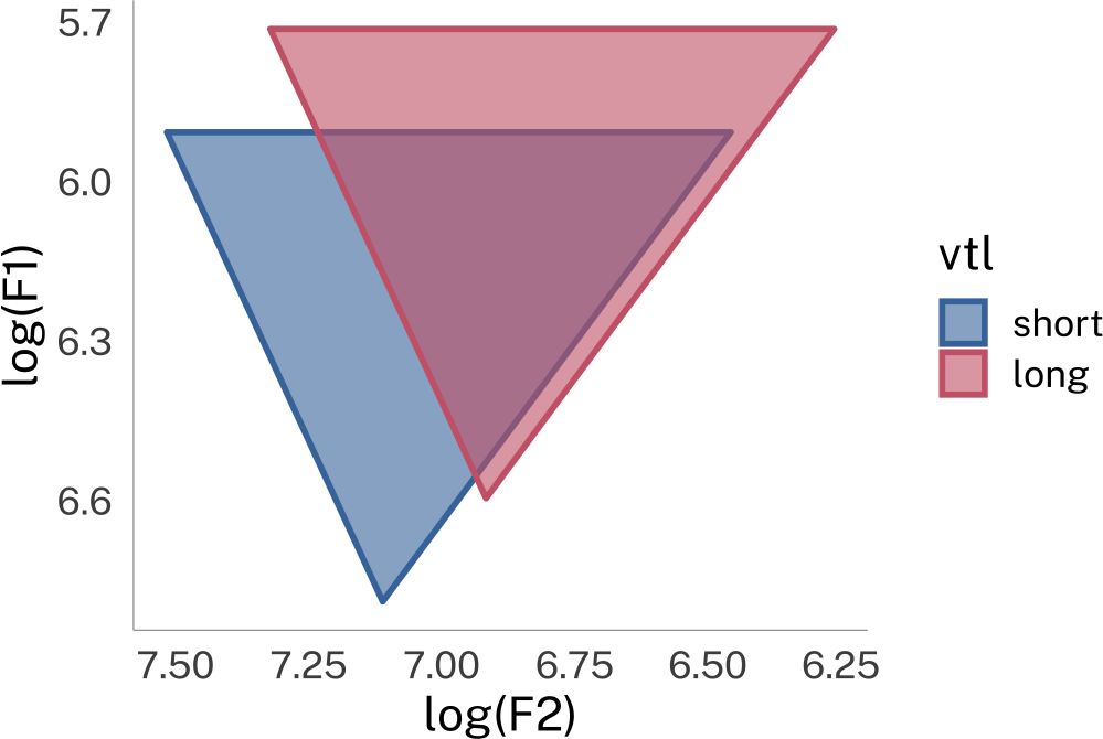

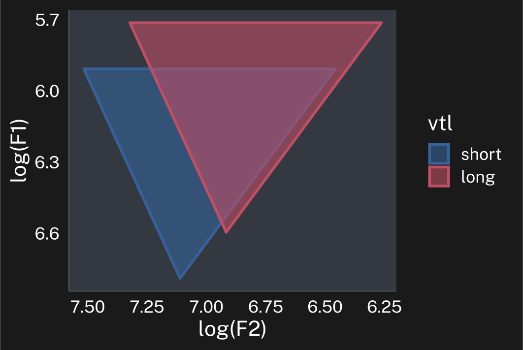
So what Nearey normalization does is

log transform the data
take the average value across all formants
subtracts that value from each token

So where \(i\) is the formant number, and \(j\) is the token number:

\[ F_{ij}' = \frac{\log F_{ij}-L}{1} \]

\[ L = \frac{1}{MN} \sum_{i=1}^3\sum_{j=1}^N \log F_{ij} \]

It’s possible to do this yourself using some tidyverse verbs, but it involves some pivoting between wide and long. This, combined with my work on normalizing vowel formant tracks motivated me to create the tidynorm package.

Normalizing with `{tidynorm}`

library(tidynorm)
library(ggdensity)

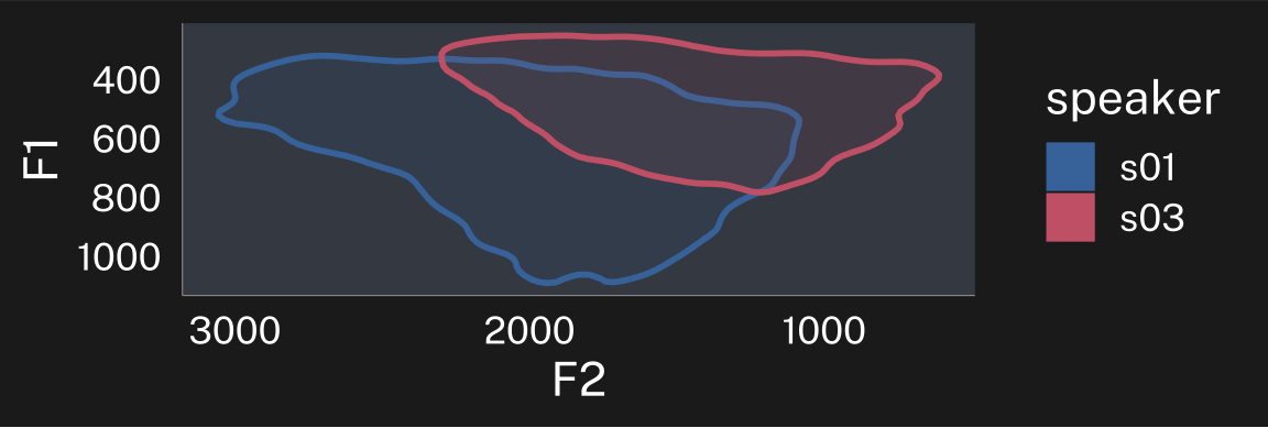
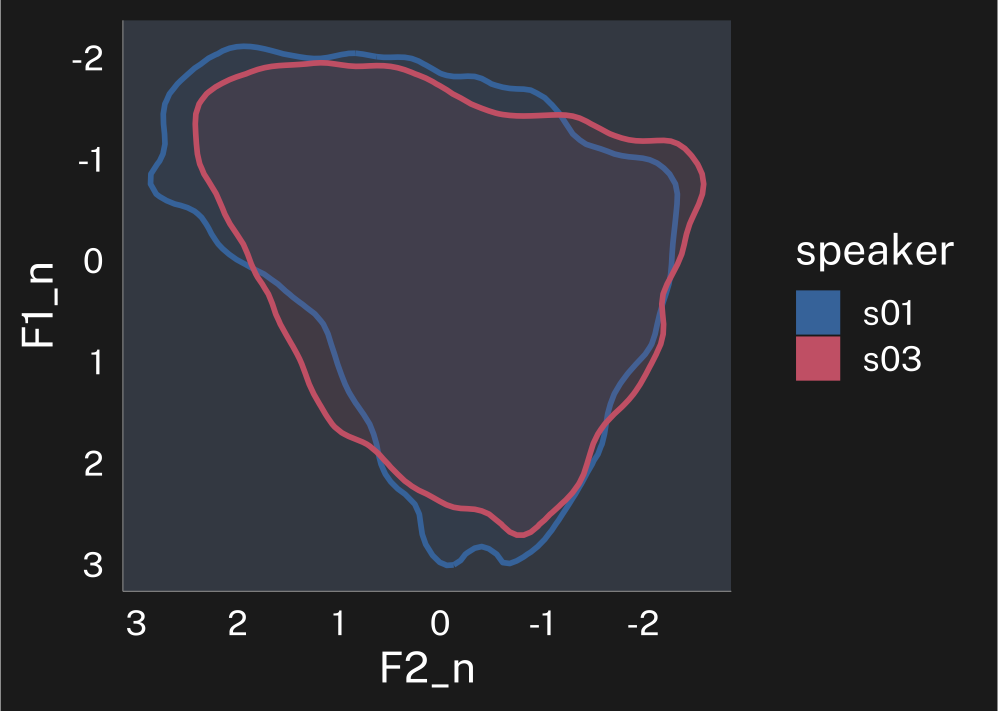
Let’s start with two speakers’ unnormalized data

plotting code

speaker_data |> 
  ggplot(
    aes(F2, F1, color = speaker)
  ) +
  stat_hdr(
    probs = 0.95,
    aes(fill = speaker),
    linewidth = 1
  )+
  scale_x_reverse() +
  scale_y_reverse() +
  guides(
    alpha = "none"
  )+
  coord_fixed()->p_unnorm

p_unnorm
p_unnorm + theme_dark()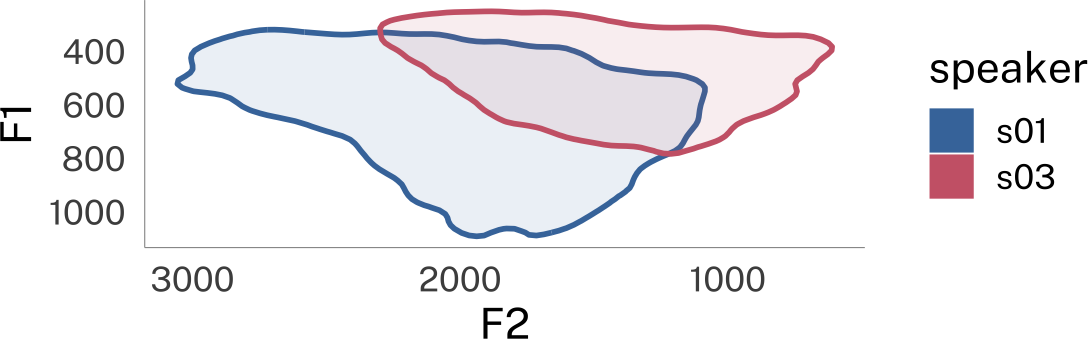

	speaker	vowel	plt_vclass	ipa_vclass	word	F1	F2	F3
1	s01	EY	eyF	ejF	OKAY	764	2088	2931
2	s01	AH	uh	ʌ	UM	700	1881	3248
3	s01	AY	ay	aj	I'M	889	1934	3120
4	s01	IH	i	ɪ	LIVED	556	1530	3462
5	s01	IH	i	ɪ	IN	612	2323	3359
6..10696
10697	s03	AH	@	ə	THE	429	1218	2352

We can implement the logic of Nearey normalization in tidynorm’s function norm_generic().

speaker_nearey <- speaker_data |>
  norm_generic(
    # the formants to normalize
    F1:F3,
    
    # provide the speaker id column
    .by = speaker,
    
    # pre calculation transformation function
    .pre_trans = log,
    
    # location calculation
    .L = mean(.formant, na.rm = T),
    
    # scope
    .by_formant = F,
    .by_token = F
  )

Normalization info
• normalized with `tidynorm::norm_generic()`
• normalized `F1`, `F2`, and `F3`
• normalized values in `F1_n`, `F2_n`, and `F3_n`
• grouped by `speaker`
• within formant: FALSE
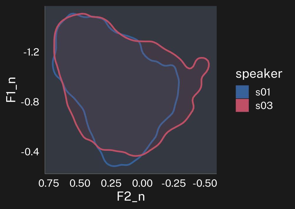
• (.formant - mean(.formant, na.rm = T))/(1)

I tried to include a helpful message describing what kind of normalization just happened. Here’s how the normalized data looks.

plotting code

speaker_nearey |> 
  ggplot(
    aes(F2_n, F1_n, color = speaker)
  ) +
  stat_hdr(
    probs = 0.95,
    aes(fill = speaker),
    linewidth = 1
  )+
  scale_x_reverse() +
  scale_y_reverse() +
  guides(
    alpha = "none"
  )+
  coord_fixed()->p_nearey

p_nearey
p_nearey + theme_dark()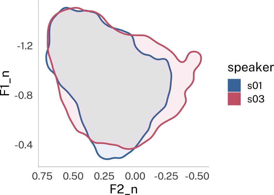

Implementing Lobanov

The Lobanov normalization technique (Lobanov 1971) essentially z-scores each formant (\(L\) = the mean, \(S\) = the standard deviation). We can see how that logic can be implemented in norm_generic() as well.

speaker_lobanov <- speaker_data |> 
  norm_generic(
    # the formants to normalize
    F1:F3,
    
    # provide the speaker id column
    .by = speaker,
    
    # location calculation
    .L = mean(.formant, na.rm = T),
    
    # scale calculation
    .S = sd(.formant, na.rm = T),
    
    # scope
    .by_formant = T,
    .by_token = F
  )

Normalization info
• normalized with `tidynorm::norm_generic()`
• normalized `F1`, `F2`, and `F3`
• normalized values in `F1_n`, `F2_n`, and `F3_n`
• grouped by `speaker`
• within formant: TRUE
• (.formant - mean(.formant, na.rm = T))/(sd(.formant, na.rm = T))

plotting code

speaker_lobanov |> 
  ggplot(
    aes(F2_n, F1_n, color = speaker)
  ) +
  stat_hdr(
    probs = 0.95,
    aes(fill = speaker),
    linewidth = 1
  )+
  scale_x_reverse() +
  scale_y_reverse() +
  guides(
    alpha = "none"
  )+
  coord_fixed()->p_lobanov

p_lobanov
p_lobanov + theme_dark()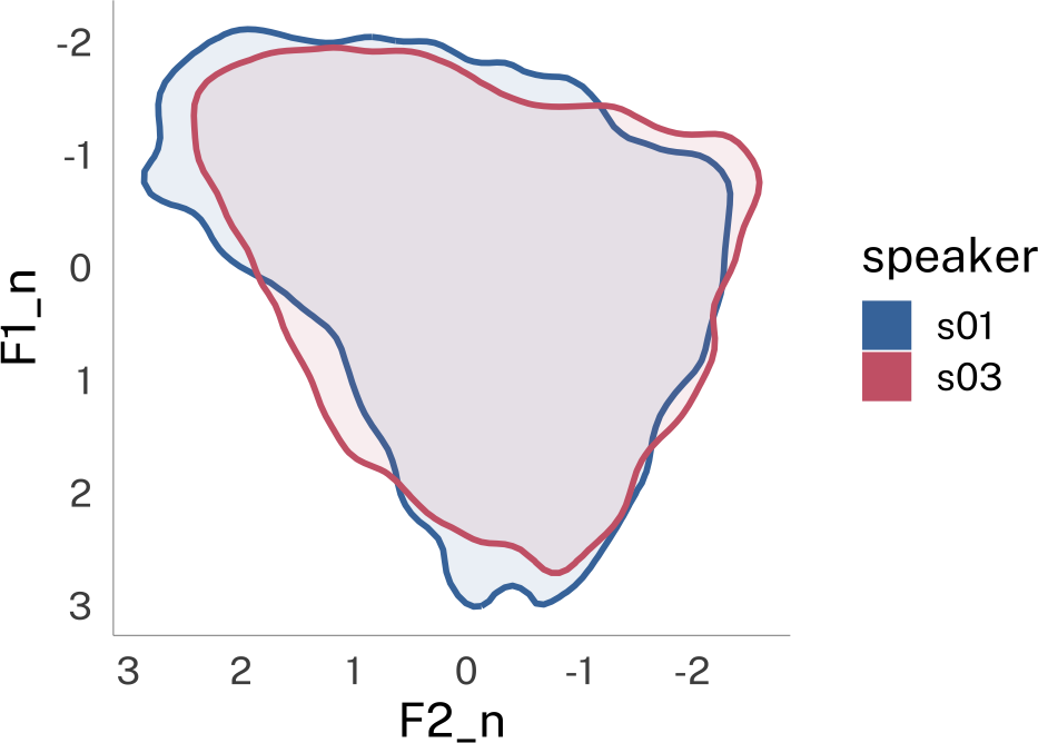

Convenience functions

Instead of needing to write out the centering and scaling functions yourself every time, I’ve included convenience functions for some established normalization methods, including

They’re all just wrappers around norm_generic(), so if you’re looking for some inspiration implementing your own normalization method, have a look at the source to see how I implemented these.

We can apply multiple normalization methods to the same data set by chaining them.

speaker_multi <- speaker_data |> 
  norm_nearey(
    F1:F3,
    .by = speaker,
    .silent = TRUE
  ) |> 
  norm_lobanov(
    F1:F3,
    .by = speaker, 
    .silent = TRUE
  ) |> 
  norm_deltaF(
    F1:F3,
    .by = speaker, 
    .silent = T
  )

If you’ve lost track of which normalization methods you’ve used, and where the normalized values have gone, you can print an information message with check_norm().

check_norm(speaker_multi)

Normalization Step
• normalized with `tidynorm::norm_nearey()`
• normalized `F1`, `F2`, and `F3`
• normalized values in `F1_lm`, `F2_lm`, and `F3_lm`
• grouped by `speaker`
• within formant: FALSE
• (.formant - mean(.formant, na.rm = T))/(1)


Normalization Step
• normalized with `tidynorm::norm_lobanov()`
• normalized `F1`, `F2`, and `F3`
• normalized values in `F1_z`, `F2_z`, and `F3_z`
• grouped by `speaker`
• within formant: TRUE
• (.formant - mean(.formant, na.rm = T))/(sd(.formant, na.rm = T))


Normalization Step
• normalized with `tidynorm::norm_deltaF()`
• normalized `F1`, `F2`, and `F3`
• normalized values in `F1_df`, `F2_df`, and `F3_df`
• grouped by `speaker`
• within formant: FALSE
• (.formant - 0)/(mean(.formant/(.formant_num - 0.5), na.rm = T))

Normalizing Formant Tracks

While I think the advice I have for normalizing formant tracks is good, I admit it’s fairly complex. So I’ve also implemented formant track normalization methods:

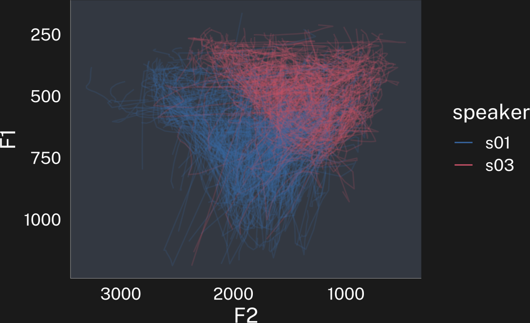
Let’s look at one of them in action on formant track data.

plotting code

speaker_tracks |>   
  filter(
    .by = c(speaker, id),
    !any(F1 > 1200)
  ) ->
  speaker_tracks

speaker_tracks |> 
  ggplot(
    aes(F2, F1, color = speaker)
  )+
  geom_path(
    alpha = 0.2,
    aes(group = interaction(speaker, id))
  )+
  guides(
    color = guide_legend(override.aes = list(alpha = 1))
  )+
  scale_x_reverse()+
  scale_y_reverse() -> p
p
p + theme_dark()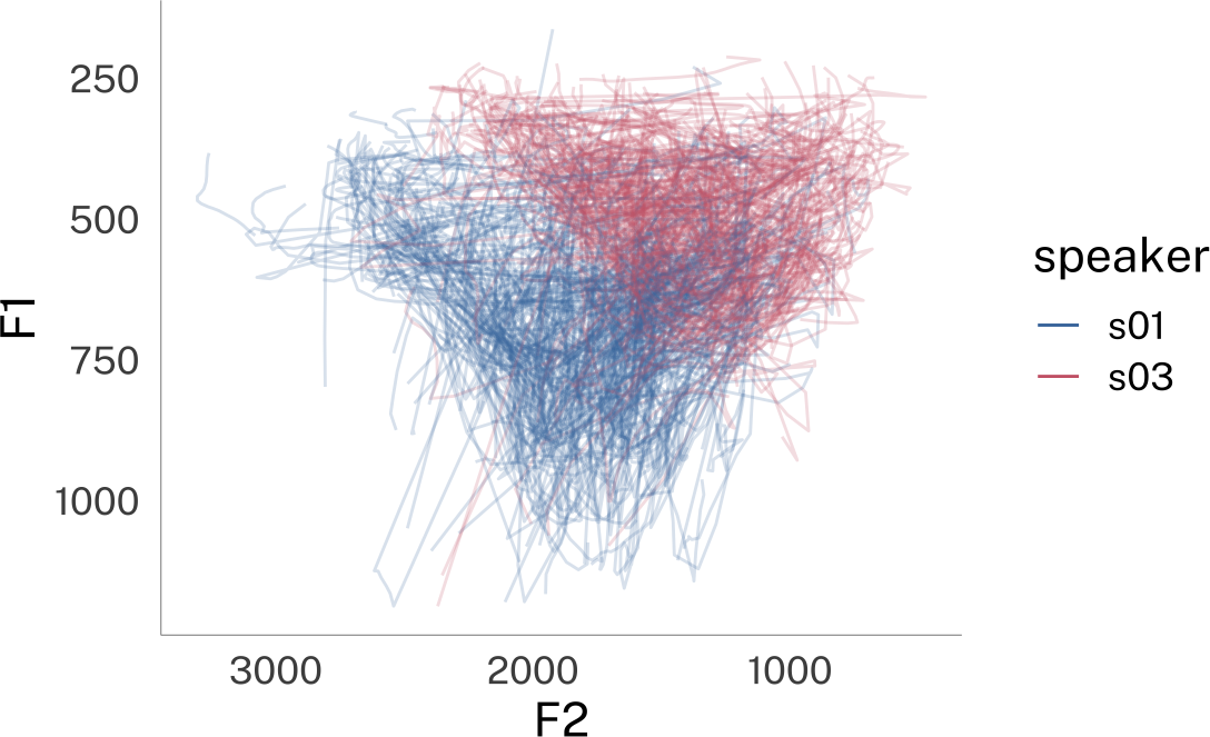

	speaker	id	vowel	plt_vclass	word	t	F1	F2	F3
1	s01	0	EY	eyF	OKAY	32.39	754	2145	2913
2	s01	0	EY	eyF	OKAY	32.40	719	2155	2913
3	s01	0	EY	eyF	OKAY	32.41	752	2115	2914
4	s01	0	EY	eyF	OKAY	32.42	762	2087	2931
5	s01	0	EY	eyF	OKAY	32.43	738	2088	2933
6..19159
19160	s03	818	UW	Tuw	TO	406.66	275	1336	2364

In addition to identifying the speaker ID column, we also need to provide a column that uniquely identifies each token (in this data set, id) and we can provide an optional column of time information.¹

speaker_track_lobanov <- speaker_tracks |> 
  norm_track_lobanov(
    # the formants to normalize
    F1:F3,
    
    # provide the speaker id column
    .by = speaker,
    
    # provide the token id column
    .token_id_col = id,
    
    # provide a time column
    .time_col = t
  )

Normalization info
• normalized with `tidynorm::norm_track_lobanov()`
• normalized `F1`, `F2`, and `F3`
• normalized values in `F1_z`, `F2_z`, and `F3_z`
• token id column: `id`
• time column: `t`
• grouped by `speaker`
• within formant: TRUE
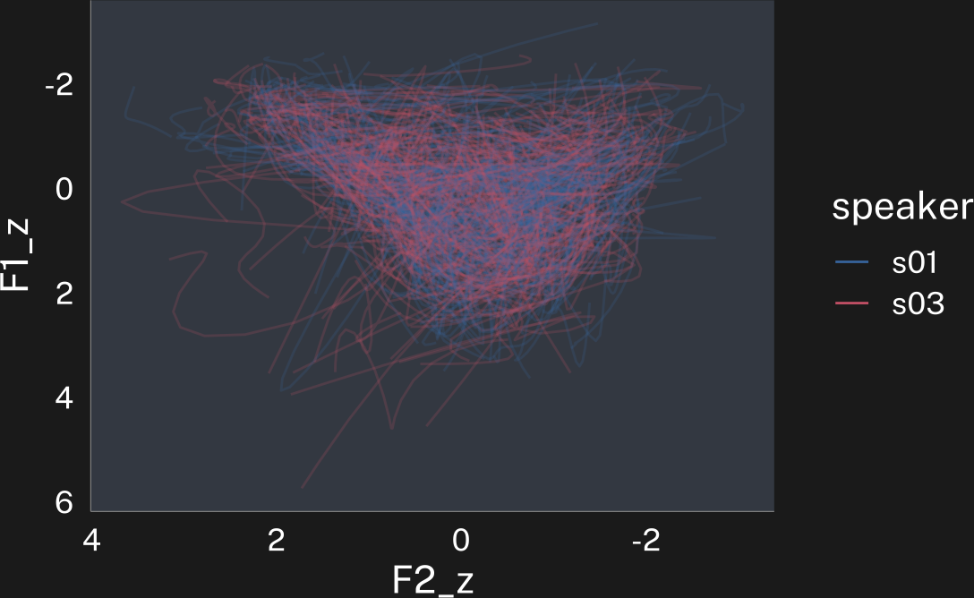
• (.formant - mean(.formant, na.rm = T))/sd(.formant, na.rm = T)

plotting code

speaker_track_lobanov |> 
  ggplot(
    aes(F2_z, F1_z, color = speaker)
  )+
  geom_path(
    alpha = 0.2,
    aes(group = interaction(speaker, id))
  )+
  guides(
    color = guide_legend(override.aes = list(alpha = 1))
  )+
  scale_x_reverse()+
  scale_y_reverse() -> p

p
p + theme_dark()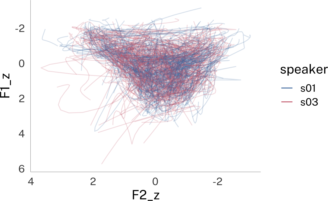

Extending `{tidynorm}`

If there is a normalization method you really like, or are just interested in, and aren’t sure how to implement it in tidynorm, add an issue (ideally with a reference or some math) on the github issues page.

Closing thoughts

This was a complex, but really enjoyable package to write. In addition to wrapping my head around “tidy evaluation”, there was a lot of conceptual work in figuring out how to implement one consistent data processing workflow in norm_generic() that could carry out the normalization methods that have been described in the literature, each in their own way. Something like

Take each formant column and z-score it.

is pretty straightforward, but something like

Transform Hz into Bark, then for each token, subtract the third formant from the first and second formants.

is a little trickier to include in the same workflow.

The tidynorm method most different from the method as described in the literature is norm_wattfab(). As described by Watt and Fabricius (2002), the method involves calculating the means of corner vowels. Doing that inside of a tidynorm workflow isn’t impossible, but would sacrifice a lot of generality, and would require users to provide a vowel-class column name every time (since I can’t assume what everyone’s data columns are called). Instead, I went for the shortcut method also used by Johnson (2020), and calculated their \(S\) values based on the mean across each formant.

I might revisit that in the future, but it would require a much more hands-on approach from the user than the other convenience functions currently do.

References

Johnson, Keith. 2020. “The ΔF Method of Vocal Tract Length Normalization for Vowels.” Laboratory Phonology: Journal of the Association for Laboratory Phonology 11 (11): 10. https://doi.org/10.5334/labphon.196.

Lobanov, Boris. 1971. “Classification of Russian Vowels Spoken by Different Listeners.” Journal of the Acoustical Society of America 49: 606–8. https://doi.org/10.1121/1.1912396.

Nearey, Terrance M. 1978. “Phonetic Feature Systems for Vowels.” PhD thesis, University of Alberta.

Watt, Dominic, and Anne Fabricius. 2002. “Evaluation of a Technique for Improving the Mapping of Multiple Speakers’ Vowel Spaces in the F1 F2 Plane.” Leeds Working Papers in Linguistics and Phonetics 9: 159–73.

Footnotes

By default, these track normalization methods will also slightly smooth the formant tracks. But if you don’t want that, you can pass it .order = NA.↩︎

Reuse

CC-BY-SA 4.0

Citation

BibTeX citation:

@online{fruehwald2025,
  author = {Fruehwald, Josef},
  title = {Introducing Tidynorm},
  series = {Væl Space},
  date = {2025-06-16},
  url = {https://jofrhwld.github.io/blog/posts/2025/06/2025-06-16_introducing-tidynorm/},
  langid = {en}
}

For attribution, please cite this work as:

Fruehwald, Josef. 2025. “Introducing Tidynorm.” Væl Space. June 16, 2025. https://jofrhwld.github.io/blog/posts/2025/06/2025-06-16_introducing-tidynorm/.

What is speaker vowel normalization?

Normalization methods

Normalizing with {tidynorm}

Implementing Lobanov

Convenience functions

Normalizing Formant Tracks

Extending {tidynorm}

Closing thoughts

References

Footnotes

Reuse

Citation

Normalizing with `{tidynorm}`

Extending `{tidynorm}`