Thinking About Hierarchical Variance Parameters

I’m still thinking about priors, distributions, and logistic regressions. The fact that a fairly broad normal distribution in logit space turns into a bimodal distribution in probability space has got me thinking about the standard deviation of random effects in logistic regression. Specifically, what happens in cases where the population of individuals may be bimodal

library(tidyverse)
library(brms)
library(tidybayes)
library(marginaleffects)

library(gt)

source(here::here("_defaults.R"))

seed <- 2023-6-29

set.seed(seed)

Simulating some data

I’ll kick things off with simulating some data. Our predictor variable will be just randomly sampled from ~normal(0,1), so it’ll handily already be z-scored. I’ll also go for a slope in logit space of 1, so logit(y) = x.

I’ll treat each point I’ve sampled for X as belonging to an individual, or subject, grouping variable, and each individual’s personal probability will be sampled from a beta distribution. I’ll simulate two possibilities here, one where individuals are kind of closely clustered near each other, and another where they’re pretty strongly bifurcated close to 0 and 1.¹

tibble(
  x = rnorm(100),
  logit = x,
  prob = plogis(logit)
) |> 
  mutate(
    individual = row_number(),
    subj_prob_low = rbeta(
      n = n(), 
      prob * 0.25, 
      (1-prob) * 0.25
    ),
    subj_prob_high = rbeta(
      n = n(), 
      prob * 7, 
      (1-prob) * 7
      )
  )->
  sim_params

sim_params |> 
  pivot_longer(
    starts_with("subj_prob")
  ) |> 
  mutate(
    name = case_when(
      name == "subj_prob_high" ~ "unimodal",
      name == "subj_prob_low" ~ "bifurcated"
    )
  ) |> 
  ggplot(aes(x, value))+
    geom_point()+
    labs(title = "subject-level probabilities",
         y = "prob")+
    scale_x_continuous(
      breaks = seq(-2,2, by = 2)
    ) +  
    facet_wrap(~name)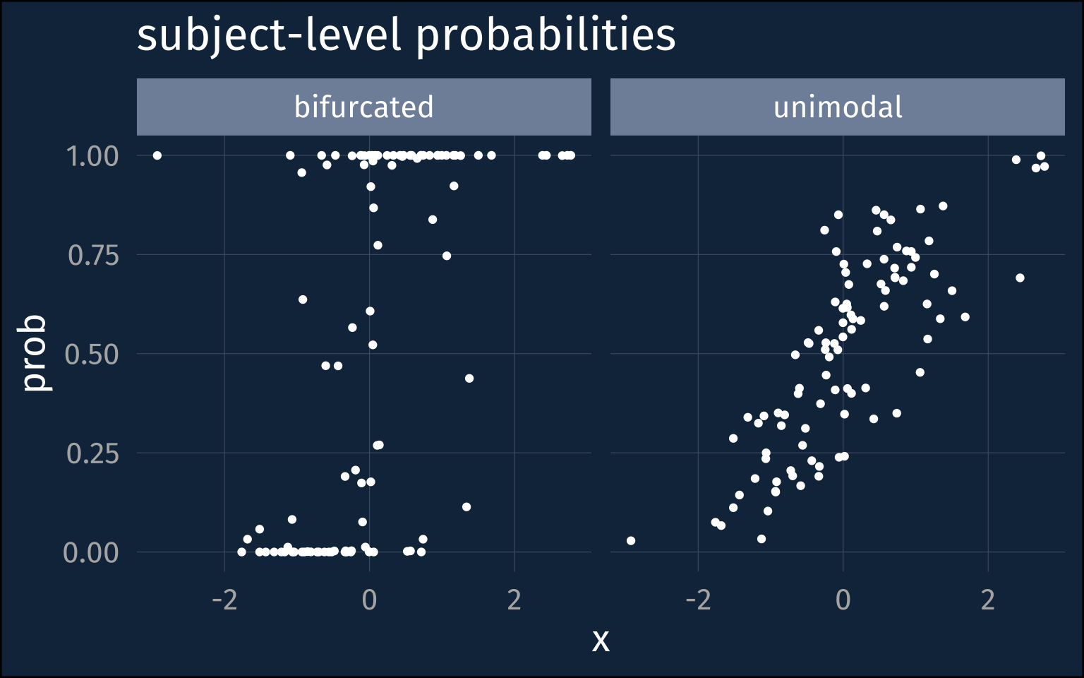

Figure 1: Probabilities for individuals

For each of these probabilities, I’ll simulate 50 binomial observations.

sim_params |> 
  rowwise() |> 
  mutate(
    obs = list(tibble(
      y_prob_low = rbinom(n = 50, size = 1, prob = subj_prob_low),
      y_prob_high = rbinom(n = 50, size = 1, prob = subj_prob_high)
    ))
  ) |> 
  unnest(obs) ->
  sim_obs

sim_obs |> 
  pivot_longer(
    starts_with("y_"),
    names_to = "simulation",
    values_to = "observation"
  ) |> 
  mutate(
    simulation = case_when(
      simulation == "y_prob_high" ~ "unimodal",
      simulation == "y_prob_low" ~ "bifurcated"
    )
  ) |> 
  ggplot(aes(x, factor(observation))) +
    stat_sum(alpha = 0.3)+
    labs(title = "simulated observations")+
    scale_x_continuous(
      breaks = seq(-2,2, by = 2)
    ) +
    facet_wrap(~simulation)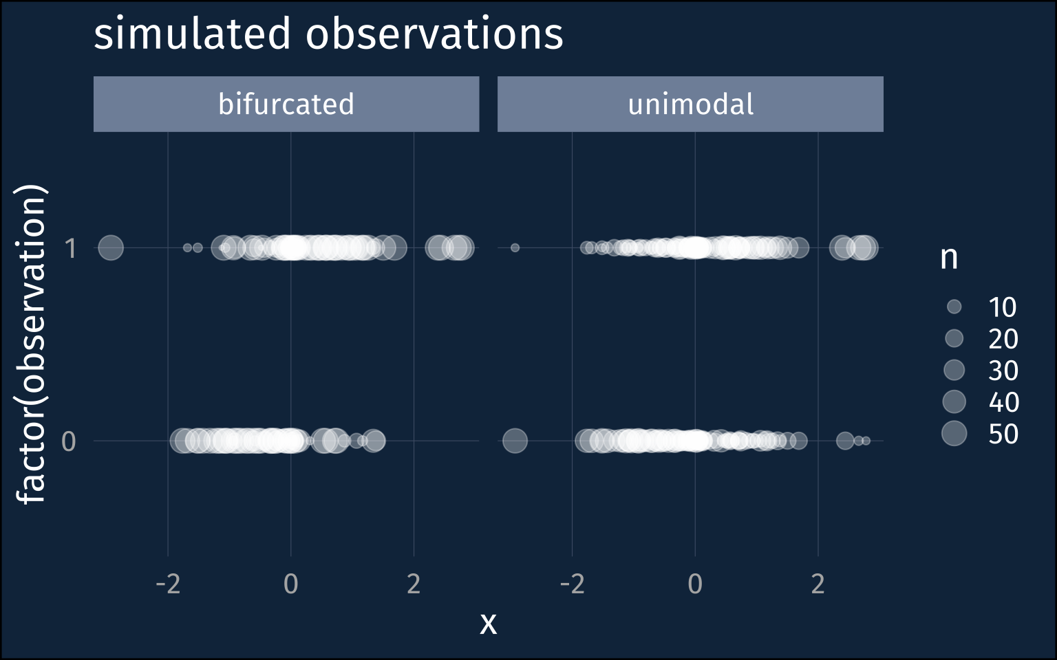

Figure 2: simulated observations

Looking at the default priors

If we take a look at the default priors a logistic model would get in brms, we can see that both the Intercept and the slope get pretty broad priors (the blank prior for the slope means it’s a flat prior).

get_prior(
  bf(y_prob_low ~ x + (1|individual)),
  data = sim_obs,
  family = bernoulli(link = "logit")
) |> 
  as_tibble() |> 
  select(prior, class, coef, group) |> 
  gt()

prior	class	coef	group
	b
	b	x
student_t(3, 0, 2.5)	Intercept
student_t(3, 0, 2.5)	sd
	sd		individual
	sd	Intercept	individual

If we real quick look at how the prior on the intercept plays out in the probability space, we get one of these bimodal distributions.

tibble(
  x = rstudent_t(1e6, df = 3, sigma = 2.5)
) |> 
  ggplot(aes(plogis(x))) +
    stat_slab(fill = ptol_red)+
    theme_no_y()+
    scale_y_continuous(
      expand = expansion(mult = 0)
    )+
    labs(title = "invlogit(student_t(3, 0, 2.5))",
         x = NULL)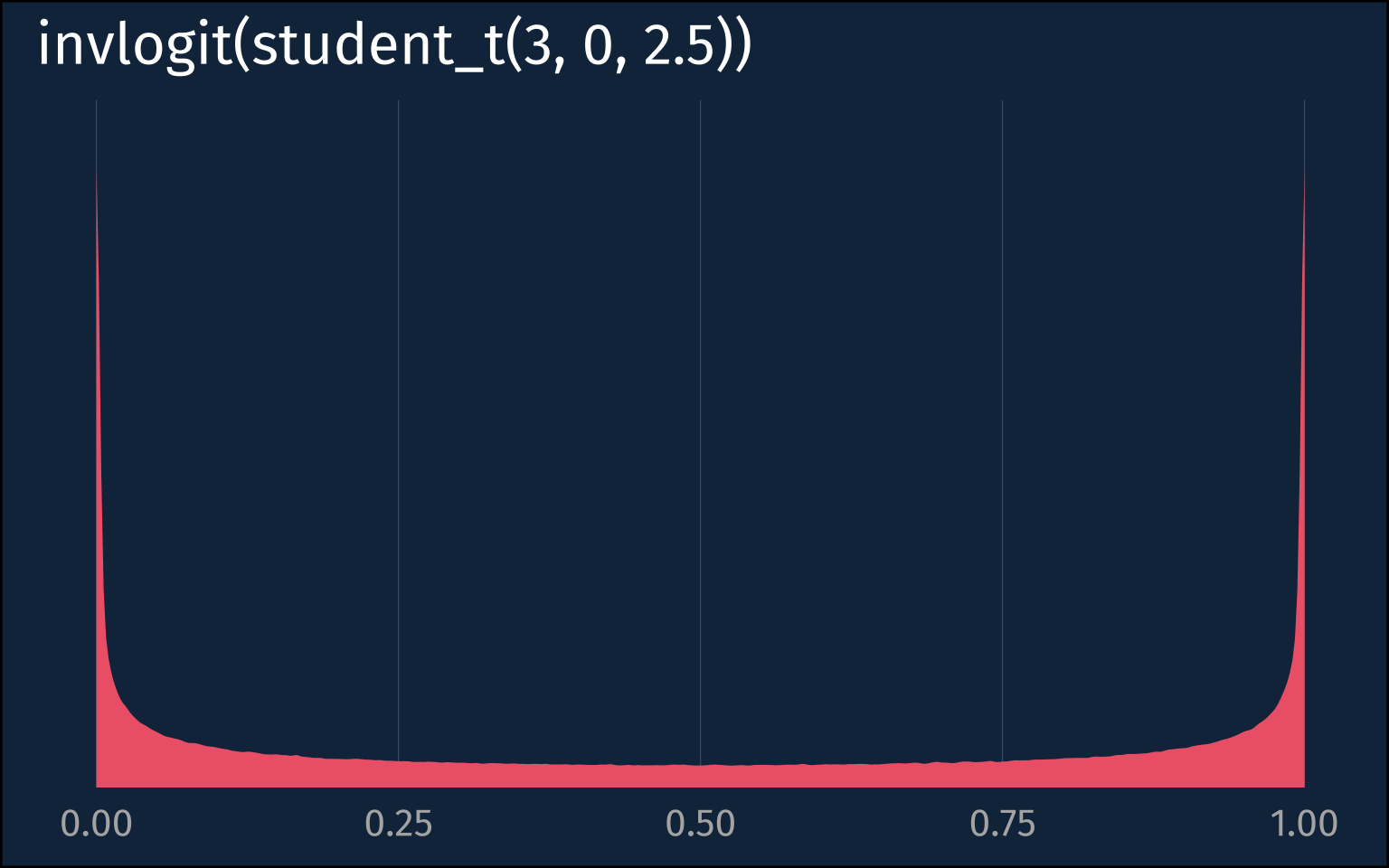

Figure 3: Student-t prior in the probability space.

So, for the intercept and slope priors, I’ll adjust them to be ~normal(0, 1.5) and ~normal(0,1), respectively.

Actually fitting the models.

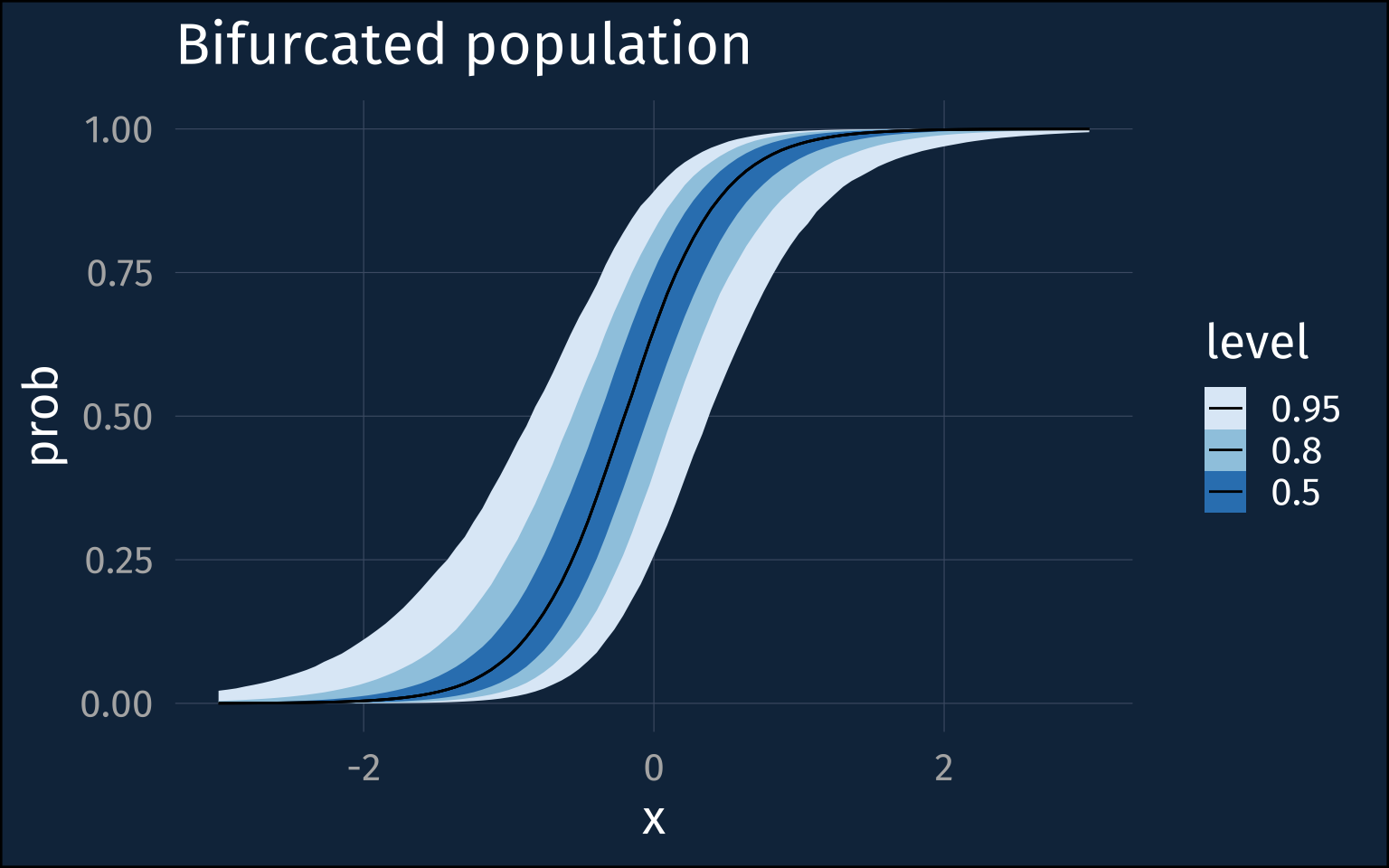
Bimodal population

First, here’s the model for the population where individuals’ probabilities were squished out towards 0 and 1.

low_mod <- brm(
  y_prob_low ~ x + (1|individual),
  data = sim_obs,
  family = bernoulli(link = "logit"),
  prior = c(
    prior(normal(0,1.5), class = "Intercept"),
    prior(normal(0,1), class = "b", coef = "x")
  ),
  cores = 4, 
  seed = seed,  
  backend = "cmdstanr",
  file = "low_mod.RDS"
) 

low_mod |> 
  gather_draws(
    `sd_.*`,
    `b_.*`,
    regex = T
  ) |> 
  mean_hdci() |> 
  select(.variable, .value, .lower, .upper) |> 
  gt() |> 
  fmt_number()

.variable	.value	.lower	.upper
b_Intercept	0.60	−1.04	2.13
b_x	3.01	1.62	4.36
sd_individual__Intercept	7.85	5.85	10.21

Things have kind of clearly gone off the rails here. The intercepts and slopes are all over the place, but that’s maybe not surprising given the trade offs the model is making between the population level slopes and the individual level probabilities. It’s worth noting that this model had no diagnostic warnings and was well converged.

low_mod |> 
  predictions(
    newdata = datagrid(x = seq(-3, 3, length = 100)),
    re_formula = NA
  ) |>
  posterior_draws() |> 
  ggplot(aes(x, draw)) +
    stat_lineribbon(linewidth = 0.5)+
    scale_fill_brewer() +
    labs(
      title = "Bifurcated population",
      y = "prob"
    )

Figure 4: The posterior fitted values.

In fact, that posterior distribution for the between-speaker sd is very extreme at about 8. If we plot the kind of distribution of individuals it suggests when the population level probability = 0.5, we get those steep walls near 0 and 1 again.

low_mod |> 
  gather_draws(
    `sd_.*`,
    regex = T
  ) |> 
  slice_sample(
    n = 10
  ) |> 
  rowwise() |> 
  mutate(
    individuals = list(tibble(
      individual = rnorm(1e5, mean = 0, sd=.value)
    ))
  ) |> 
  unnest(individuals) |> 
  ggplot(aes(plogis(individual)))+
    stat_slab(
      aes(group = factor(.value)),
      linewidth = 0.5,
      fill = NA,
      color = ptol_red
    ) +
    scale_y_continuous(expand = expansion(mult = 0))+
    labs(
      title = "Random intercepts distribution around 0.5"
    )+
    theme_no_y()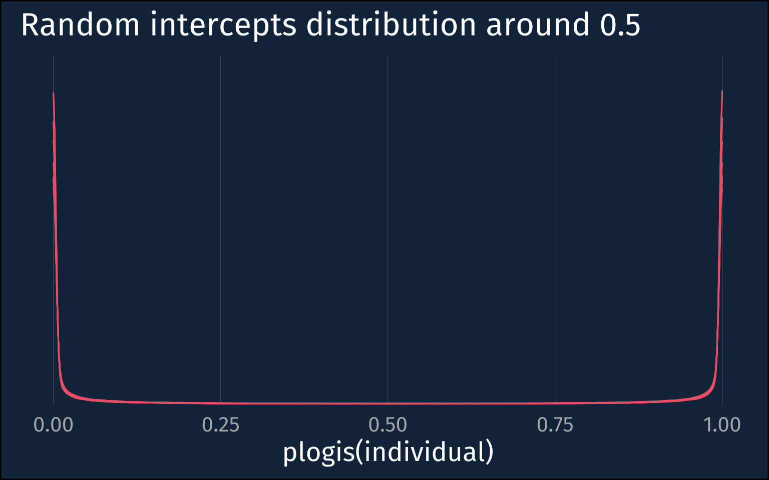

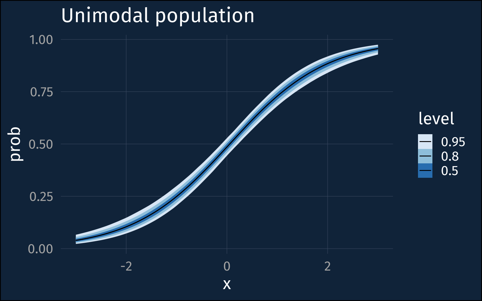
Figure 5: Implied distribution of individuals in the bifircated population.

The Unimodal Population

Let’s do it all again, but now for the population where individuals’ probabilities were clustered around the population probability.

high_mod <- brm(
  y_prob_high ~ x + (1|individual),
  data = sim_obs,
  family = bernoulli(link = "logit"),
  prior = c(
    prior(normal(0,1.5), class = "Intercept"),
    prior(normal(0,1), class = "b", coef = "x")
  ),
  cores = 4,
  adapt_delta = 0.9,
  seed = seed,
  backend = "cmdstanr",
  file = "high_mod.RDS"
) 

high_mod |> 
  gather_draws(
    `sd_.*`,
    `b_.*`,
    regex = T
  ) |> 
  mean_hdci() |> 
  select(
    .variable, .value, .lower, .upper
  ) |> 
  gt() |> 
   fmt_number(decimals = 2)

.variable	.value	.lower	.upper
b_Intercept	−0.06	−0.23	0.10
b_x	1.05	0.87	1.22
sd_individual__Intercept	0.77	0.63	0.91

The intercepts and slope posteriors are much more tight, and the inter-speaker sd posterior is <1.

high_mod |> 
  predictions(
    newdata = datagrid(x = seq(-3, 3, length = 100)),
    re_formula = NA
  ) |> 
  posterior_draws() |> 
  ggplot(aes(x, draw)) +
    stat_lineribbon(linewidth = 0.5)+
    scale_fill_brewer()+
    labs(
      title = "Unimodal population",
      y = "prob"
    )

Figure 6: Posterior fitted values for the unimodal population.

Let’s look at the implied individual level distribution around 0.5.

high_mod |> 
  gather_draws(
    `sd_.*`,
    regex = T
  ) |> 
  slice_sample(
    n = 20
  ) |> 
  rowwise() |> 
  mutate(
    individuals = list(tibble(
      individual = rnorm(1e5, mean = 0, sd=.value)
    ))
  ) |> 
  unnest(individuals) |> 
  ggplot(aes(plogis(individual)))+
    stat_slab(
      aes(group = factor(.value)),
      linewidth = 0.5,
      fill = NA,
      color = ptol_red
    ) +
    scale_y_continuous(expand = expansion(mult = 0))+
    labs(
      title = "Random intercepts distribution around 0.5"
    )+
    theme_no_y()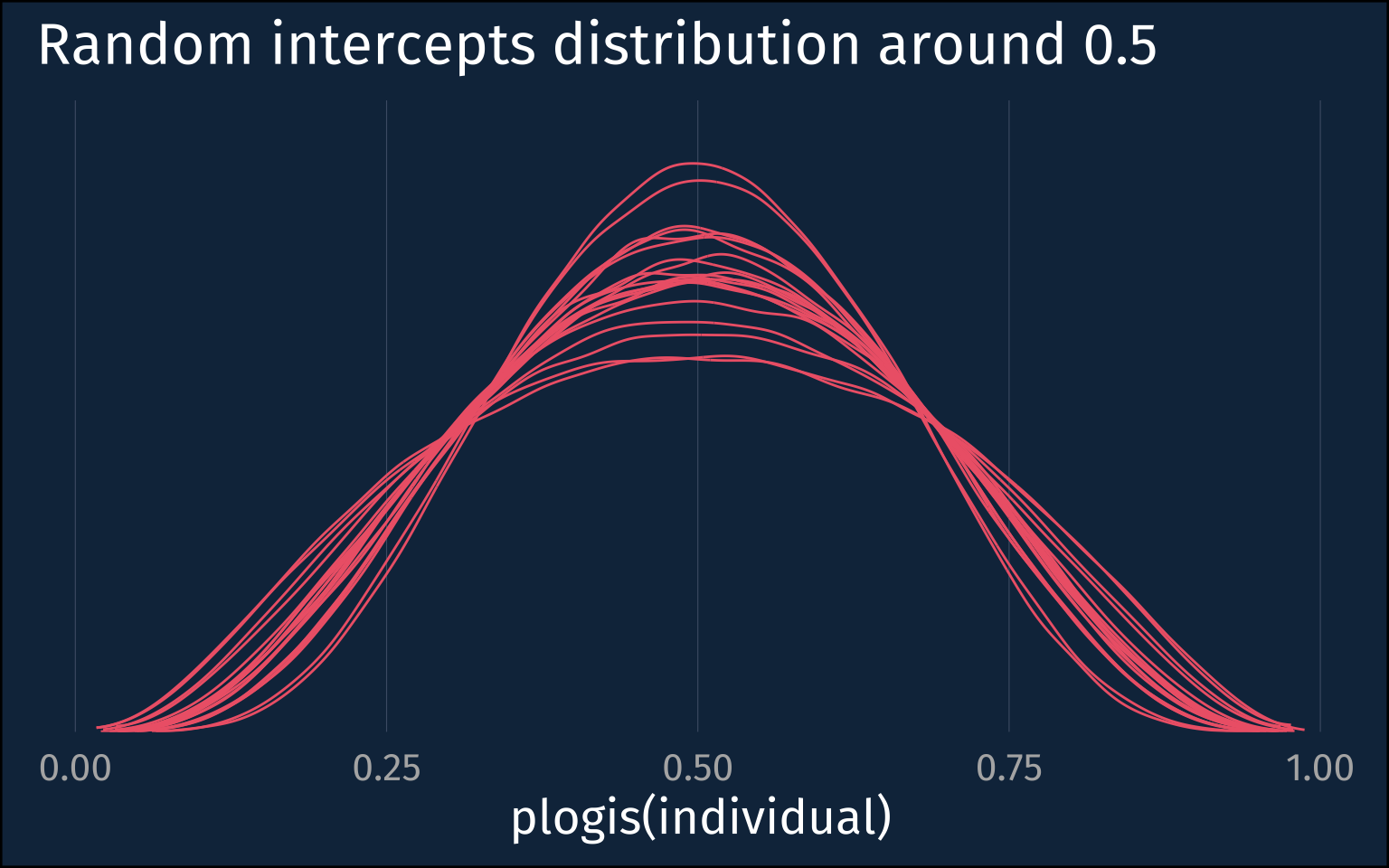

Figure 7: Implied distribution of individuals in the unimodal population.

The Upshot

Even though I’ve fit and looked at hierarchical logistic regressions before, I hadn’t stopped to think about how to interpret the standard deviation of the random intercepts before. If you’d asked me before what a large sd implied about the distribution of individuals in the probability space, I think I would have said they’d be more uniformly distributed, but actually it means they’re more bifurcated!

Also, if you’ve got a fairly bifurcated population, the population level estimates are going to get pretty wonky.

All food for thought moving forward.

Footnotes

1. I initially also tried simulating a case where individuals were strictly categorical based on the probability associated with their x, and things did not go well for the models.