
As I scroll through my feeds, I often come across a really cool looking package, or a new feature of a package, that I think looks really cool, and then I forget to go back to really kick the tires to see how it works. So I’ve decided to try to set up a workflow where I send the docs or pkgdown pages for the package to a Trello board, and then come back maybe once a month and experiment with them in a blog post.
{ggforce}, {ggdensity} and {geomtextpath}
The packages I want to mess around with today are all extensions to ggplot2, so I’ll load up the palmerpenguins dataset for experimentation.
{ggforce} and convex hulls
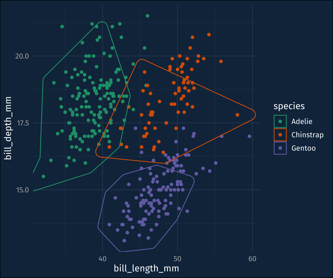
The ggforce package as the option to add a convex hull over your data (ggforce::geom_mark_hull()), kind of indicating where the data clusters are. Here’s my base plot.
plot1 <-
  penguins |>
  drop_na() |>
  ggplot(aes(bill_length_mm, bill_depth_mm, color = species))+
    geom_point()+
    scale_color_brewer(palette = "Dark2")+
    scale_fill_brewer(palette = "Dark2")
plot1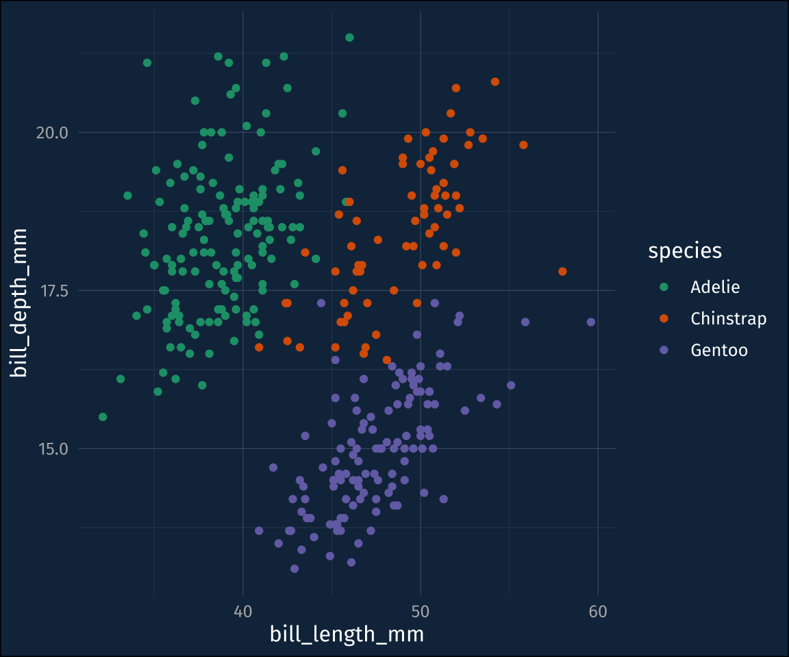
I’ll throw on the default convex hull.
plot1 +
  geom_mark_hull()
Warning: Using the `size` aesthetic in this geom was deprecated in ggplot2 3.4.0.
ℹ Please use `linewidth` in the `default_aes` field and elsewhere instead.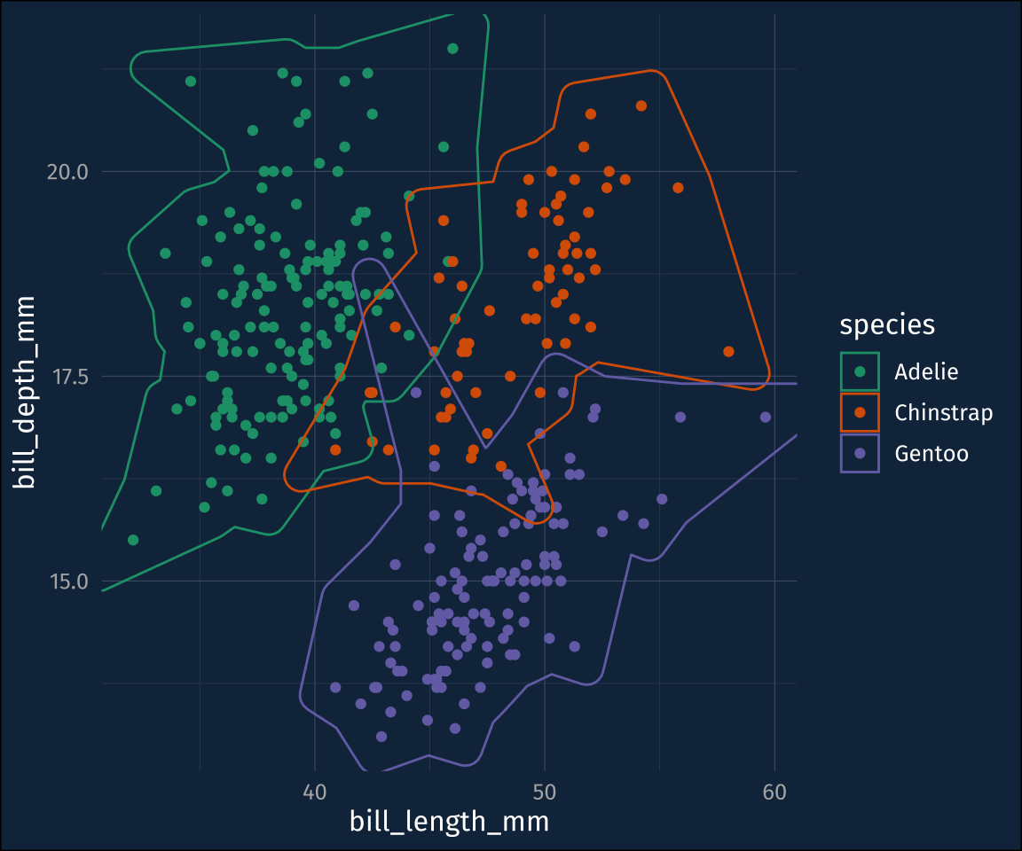
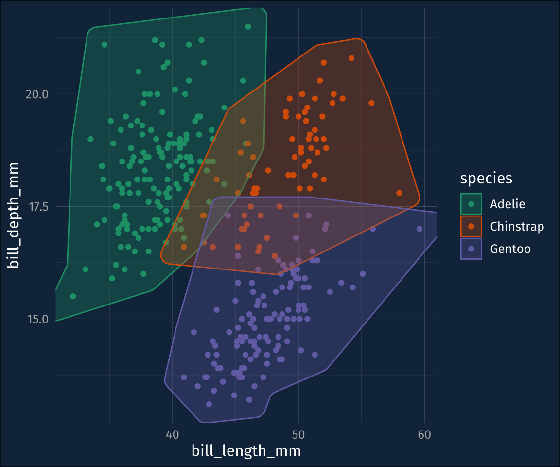
Default is ok, but for this data set, the hulls are a bit jagged. That can be adjusted with the concavity argument. I’ll also throw in a fill color.
plot1 +
  geom_mark_hull(
    concavity = 5,
    aes(
      fill = species
    )
  )
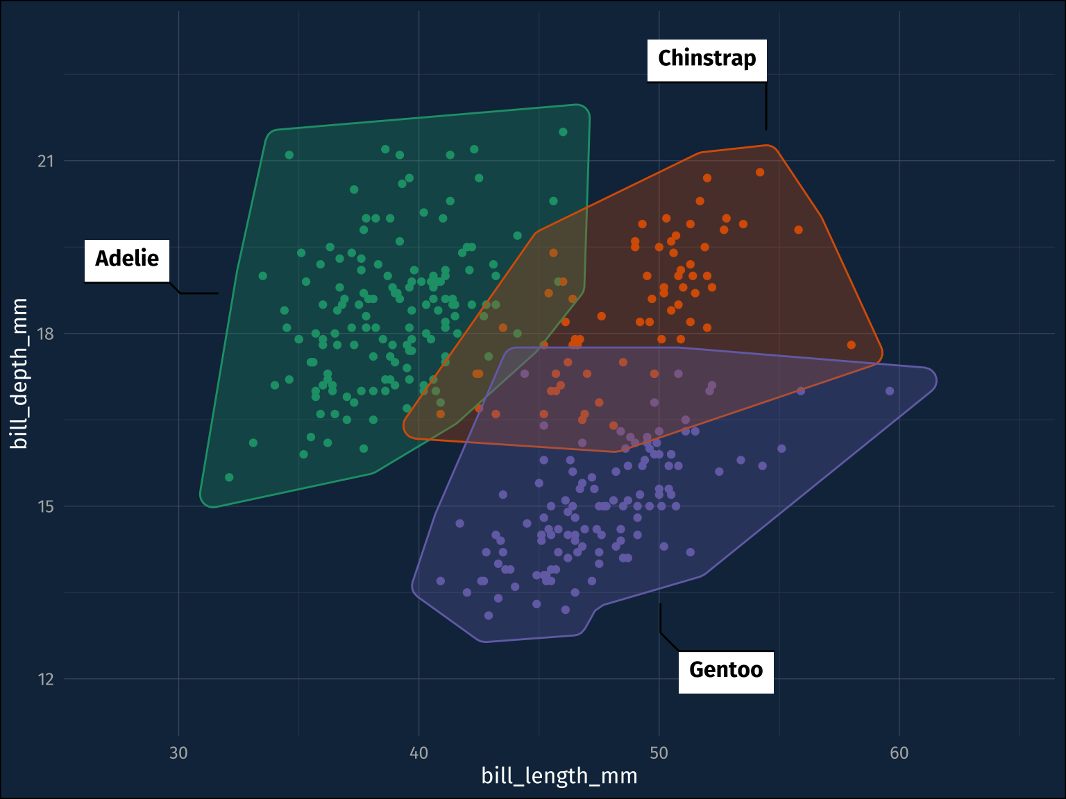
That’s better. It also comes with a mappable label and description aesthetics. Here, it seems a bit more touchy.
plot1 +
  geom_mark_hull(
    concavity = 5,
    aes(fill = species,
        label = species,
    ),
    label.family = "Fira Sans"
  )
The labels actually appear in the RStudio IDE for me, but not in the rendered page here because it wants more headroom around the plot. I’ll add that in by setting the expand arguments to ggplot::scale_y_continuous() and ggplot::scale_x_continuous(), and I’ll drop the legend while I’m at it.
plot1 +
  geom_mark_hull(
    concavity = 5,
    aes(fill = species,
        label = species,
    ),
    label.family = "Fira Sans"
  )+
  scale_y_continuous(
    expand = expansion(
      mult = c(0.25, 0.25)
    )
  )+
  scale_x_continuous(
    expand = expansion(
      mult = c(0.25, 0.25)
    )
  ) +
  guides(
    color = "none",
    fill = "none"
  )
Thoughts
I like the convex hulls as a presentational aide. It probably shouldn’t be taken as a statistical statement about, for example the degree of overlap between these three species, but is useful for outlining data points of interest.
I kind of wish this was separated out into a few different, more conventional, ggplot2 layers. It’s called a geom_ but the convex hulls are definitely stat_s. The convex hull statistic layer isn’t exposed to users, so you can’t mix-and-match convex hull estimation and the geom used to draw it. On the other hand, I can see that it’s much more souped up than a typical geom. For example, you can filter the data within the aes() mapping.
plot1 +
  geom_mark_hull(
    concavity = 5,
    aes(
      filter = sex == "female"
    )
  )
{ggdensity}
As pointed out on the ggdensity readme, there’s already a stat+geom in ggplot2 to visualize 2d density plots.
plot2 <-
  penguins |>
  drop_na() |>
  ggplot(aes(bill_length_mm, bill_depth_mm))

plot2 +
  stat_density_2d_filled()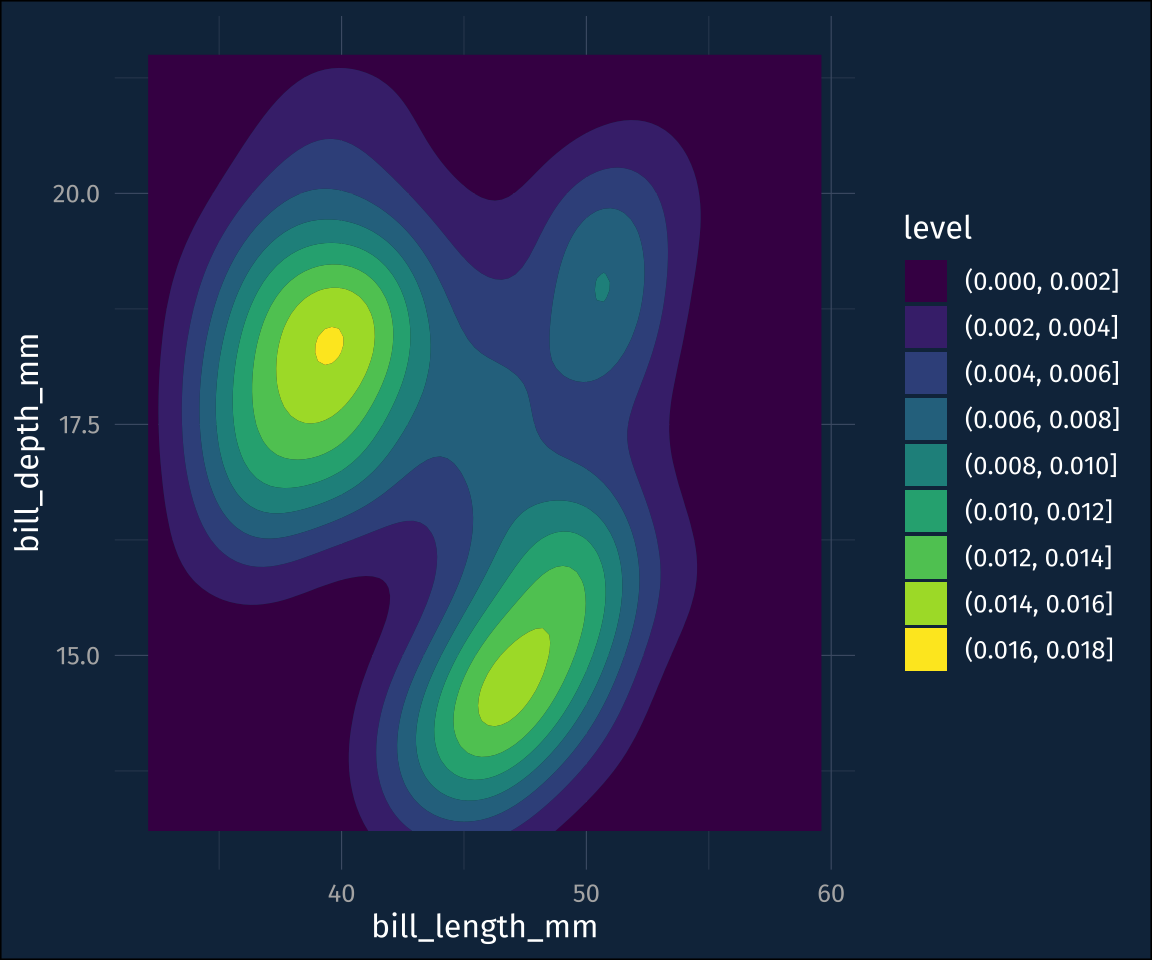
Those levels are a little hard to follow, though, which is what ggdensity::stat_hdr() is for. It will plot polygons/contours for given probability levels, of the data distribution
plot2 +
  stat_hdr()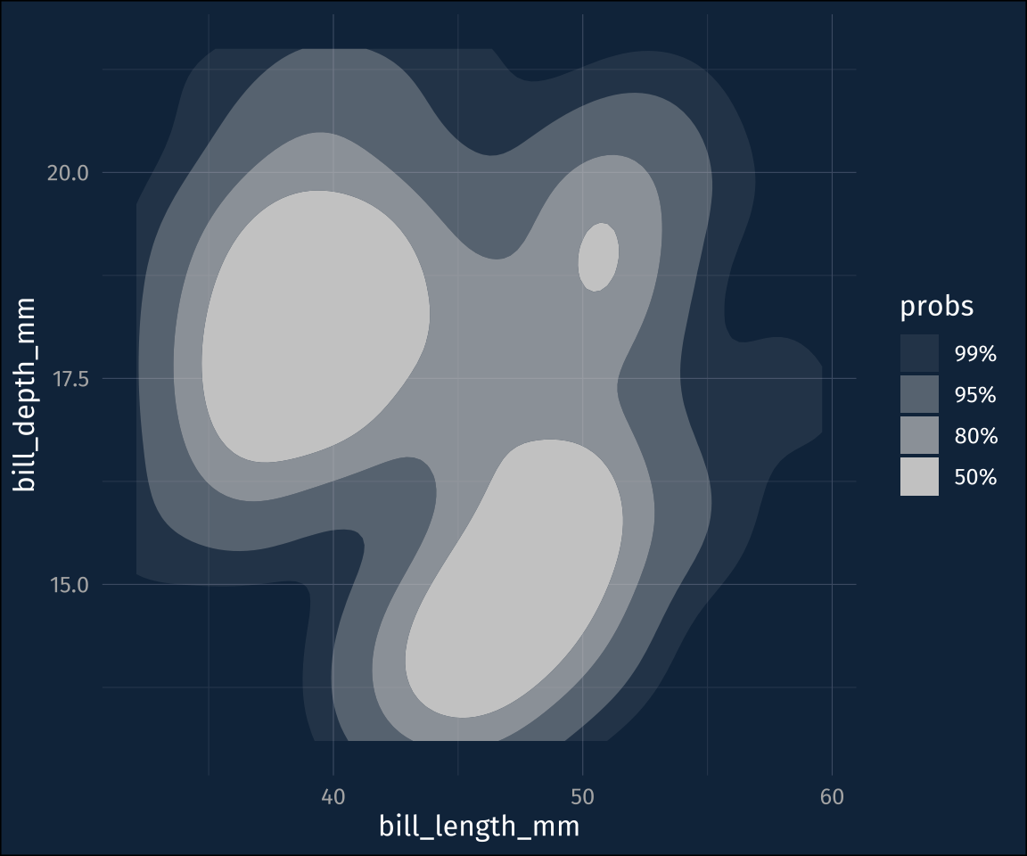
The probabilities are mapped to transparency by default, so you can map the fill color to a different dimension.
plot2 +
  stat_hdr(aes(fill = species))+
  scale_fill_brewer(palette = "Dark2")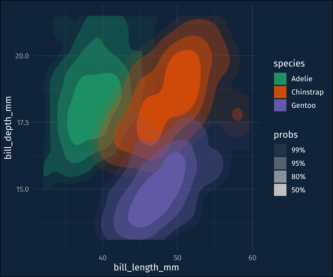
The package also has a ggdensity::stat_hdr_rug() to add density distribution rugs to plots.
plot2 +
  geom_point()+
  stat_hdr_rug(fill = "grey90")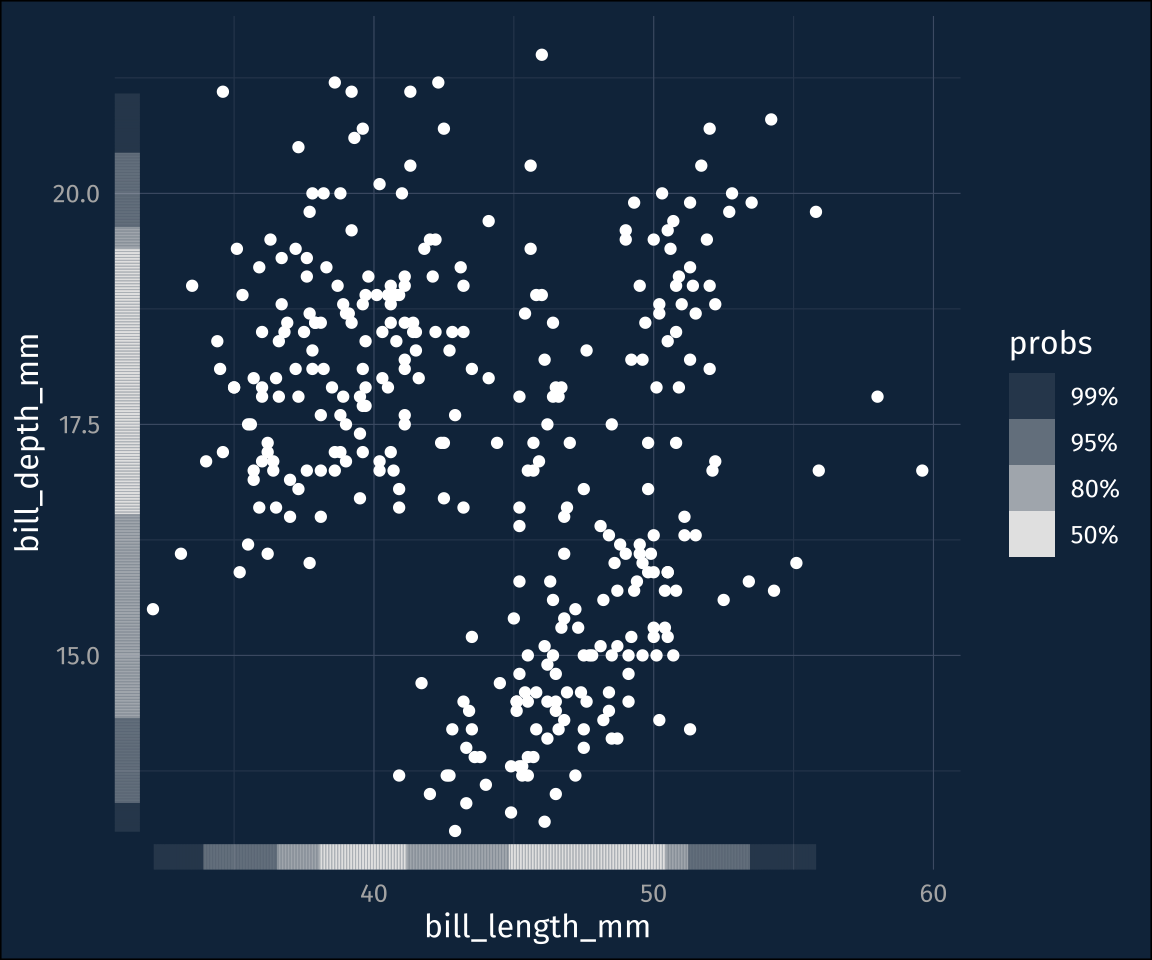
{geomtextpath}
I’ve actually been messing around with this for a bit, but geomtextpath allows you to place text along lines. There’s standalone geom_textpath() and geom_labelpath() functions, but just to stick with the penguins data, I’m going to match the textpath geom with a different stat.
plot3 <-
  penguins |>
  drop_na() |>
  ggplot(aes(bill_length_mm, bill_depth_mm, color = species))+
    scale_color_brewer(palette = "Dark2")

plot3 +
  stat_smooth(
    geom = "textpath",
    # you have to map a label aesthetic
    aes(label = species),
  ) +
  guides(color = "none")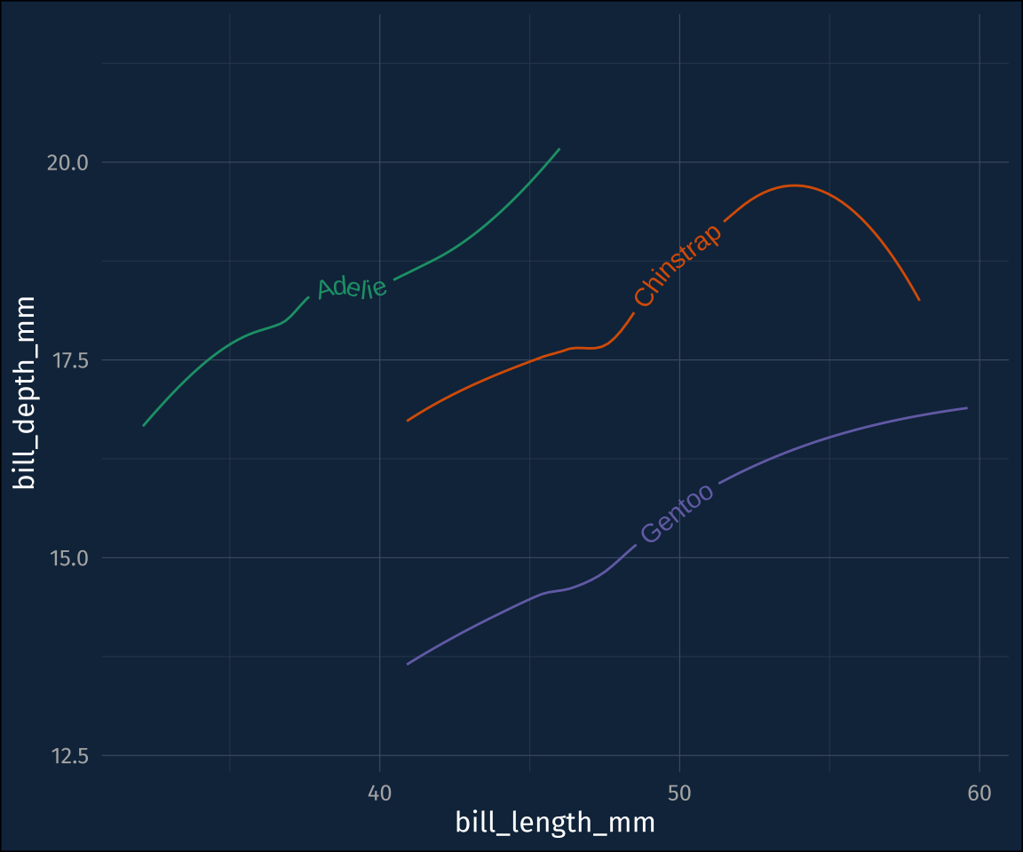
You can move the location of the text on the path back and forth by either setting or mapping hjust to a number between 0 and 1, and you can lift the text off the line with vjust.
plot3 +
  stat_smooth(
    geom = "textpath",
    # you have to map a label aesthetic
    aes(label = species),
    hjust = 0.1,
    vjust = -1
  ) +
  guides(color = "none")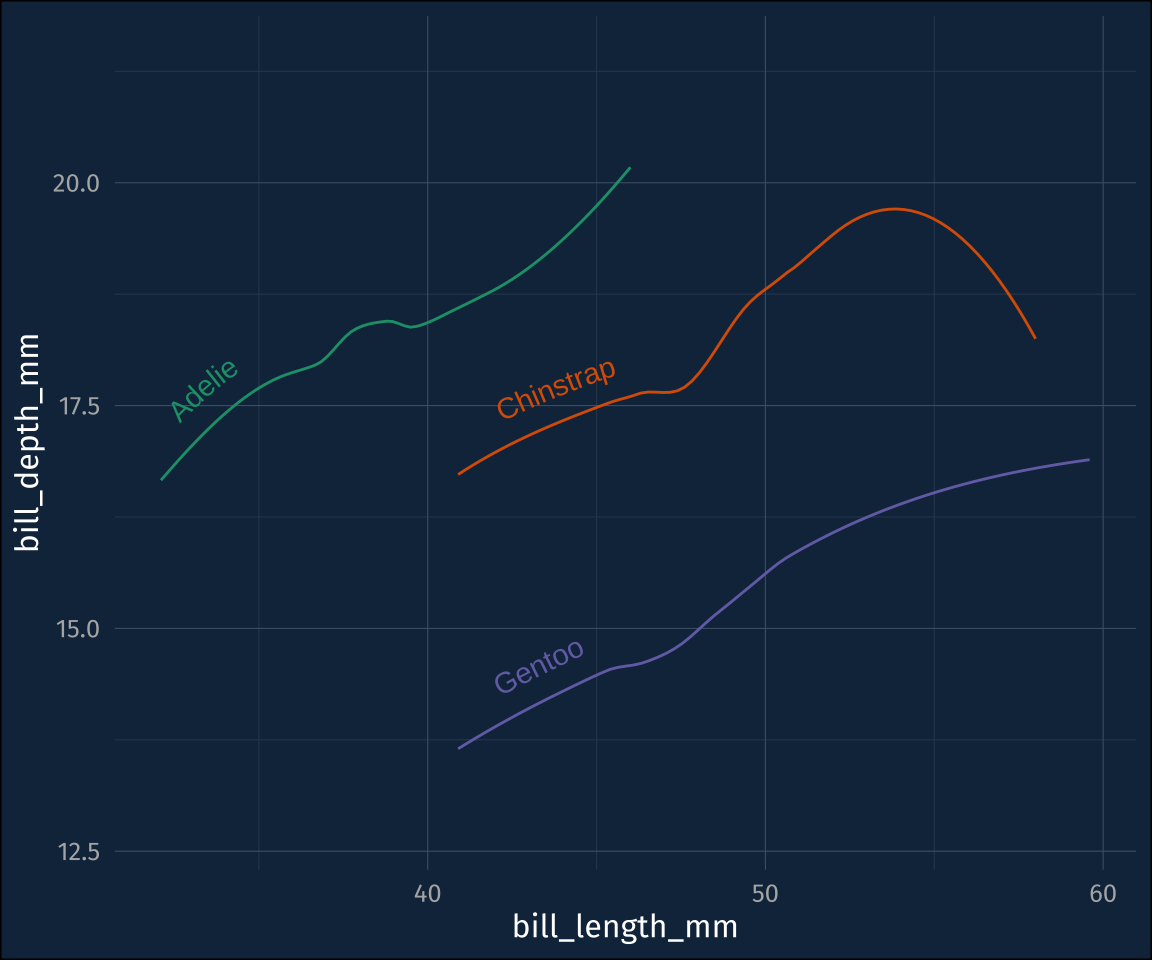
Mixing and matching statistics and these direct labels could get pretty powerful. For example, here’s the name of each species written around data ellipses.
plot3 +
  stat_ellipse(
    geom = "textpath",
    # you have to map a label aesthetic
    aes(label = species),
    hjust = 0.1
  ) +
  guides(color = "none")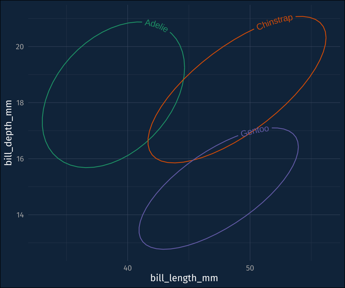
Combo {ggdensity} and {geomtextpath}
Since the ggdensity statistics are ordinary stat_, we can also combine them with textpaths to label the probability levels directly.
plot2 +
  stat_hdr_lines(
    aes(label = after_stat(probs)),
    color = "grey90",
    geom = "textpath"
  ) +
  guides(alpha = "none")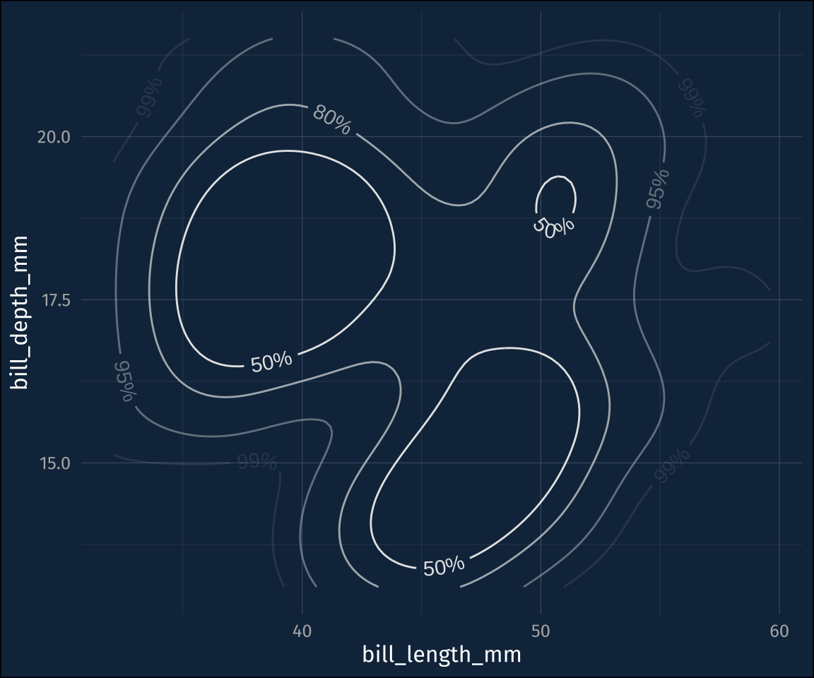
Reuse
Citation
@online{fruehwald2023,
  author = {Fruehwald, Josef},
  title = {R {Package} {Exploration} {(Jan} 2023)},
  series = {Væl Space},
  date = {2023-01-27},
  url = {https://jofrhwld.github.io/blog/posts/2023/01/2023-01-27_jan-rpackages/},
  doi = {10.59350/nbehe-t6x17},
  langid = {en}
}