Mixed Effects Models 1

Setup

Installing new packages

if(!require(broom.mixed)){
  install.packages("broom.mixed")
  library(broom.mixed)
}

if(!require(lme4)){
  install.packages("lme4")
  library(lme4)
}

if(!require(janitor)){
  install.packages("janitor")
  library(janitor)
}

Loading already installed packages

library(marginaleffects)
library(tidyverse)

Loading data for today

ey_dat <- read_csv("https://bit.ly/ey_dat")

Looking at the data

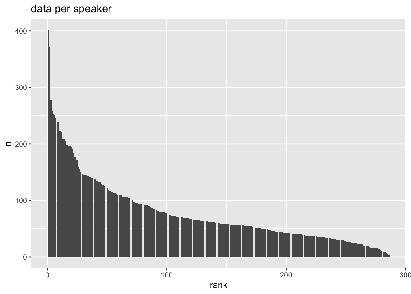
Imbalance is going to be rampant!

ey_dat |>                       
  count(speaker) |>
  mutate(
    rank = rank(
      desc(n),
      ties.method = "random"
    )                           
  ) |> 
  ggplot(aes(rank, n))+
    geom_col()+
    labs(
      title = "data per speaker"
    )

1

Getting the total number of observations per speaker.

2

Adding on a column.

3

Getting the rank of n, the number of observations.

4

We want the descending rank (that is, the largest n should get 1.

5

When two or more speakers have the same n, randomly assign the next rank, rather than giving them all the same rank.

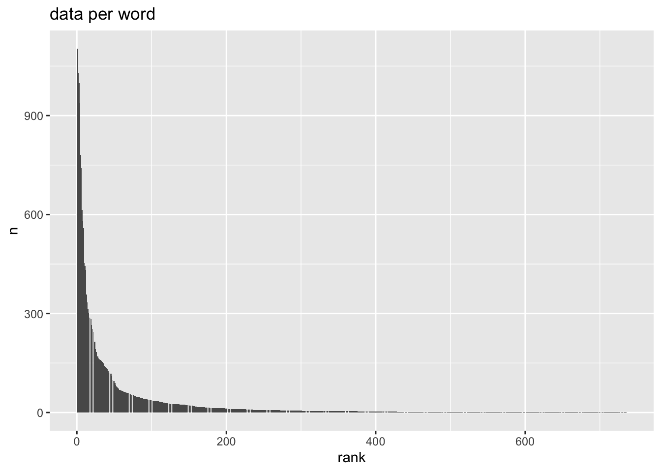
ey_dat |> 
  count(word) |> 
  mutate(
    rank = rank(
      desc(n),
      ties.method = "random"
    )
  ) |> 
  ggplot(aes(rank, n))+
    geom_col()+
    labs(
      title = "data per word"
    )

Prepare the data for modelling

ey_dat |> 
  mutate(
    dob_0 = (dob - median(dob))/25,
    log_freq = log2(frequency),
    freq_c = log_freq - median(log_freq),
    log_dur = log2(dur),
    dur_c = log_dur - median(log_dur)
  ) |> 
  drop_na()->
  ey_to_model

Modelling

“Complete Pooling”

That is, pooling all speakers’ data together.

Q: What is the effect of word frequency on F1_n?

ey_flat <- lm(F1_n ~ freq_c, data = ey_to_model)

The model parameters

tidy(ey_flat)

# A tibble: 2 × 5
  term        estimate std.error statistic  p.value
  <chr>          <dbl>     <dbl>     <dbl>    <dbl>
1 (Intercept)  -0.384    0.00352    -109.  0       
2 freq_c        0.0126   0.00126      10.0 1.60e-23

The fitted values

Step 1, get a reasonable range of freq_c values to get predictions between.

freq_range <- quantile(
  ey_to_model$freq_c, 
  probs = c(0.025, 0.975)
)

freq_range

     2.5%     97.5% 
-6.306671  3.563938 

Step 2, get the predictions

predictions(
  model = ey_flat,
  newdata = datagrid(
    freq_c = seq(freq_range[1], freq_range[2], length = 50)
  )
)  |> 
  as_tibble() ->
  ey_flat_predicted

1

marginaleffects::predictions()

2

The model we’re getting predicted values from.

3

Using marginaleffects::datagrid() to create an “grid” of data to make predictions for.

4

We want predictions from the beginning to the end of freq_range with 50 total predictions.

5

Converting the result to a tibble.

ey_flat_predicted |> 
  ggplot(aes(freq_c, estimate))+
    geom_ribbon(
      aes(ymin = conf.low, ymax = conf.high),
      alpha = 0.6
    )+
    geom_line()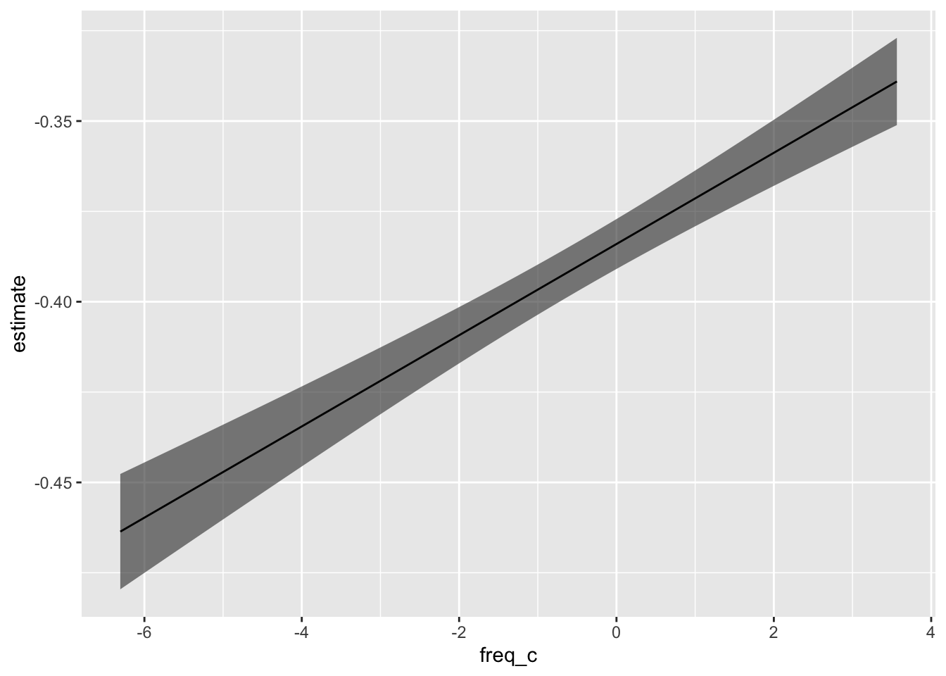

No Pooling

One model per speaker.

Fitting the models

Step 1: “Nest” the speaker data.

ey_to_model |> 
  group_by(speaker) |> 
  nest() -> 
  ey_nested

head(ey_nested)

# A tibble: 6 × 2
# Groups:   speaker [6]
  speaker   data               
  <chr>     <list>             
1 PH00-1-1- <tibble [110 × 15]>
2 PH00-1-2- <tibble [141 × 15]>
3 PH00-1-3- <tibble [192 × 15]>
4 PH00-1-4- <tibble [125 × 15]>
5 PH00-1-5- <tibble [204 × 15]>
6 PH02-1-1- <tibble [62 × 15]> 

Step 2: Write a little function to fit a linear model to a data frame

fit_lm <- function(df){
  lm(F1_n ~ freq_c, data = df)
}

Step 3: purrr:map() that function over the data column.

ey_nested |> 
  mutate(models = map(data, fit_lm)) ->
  ey_nested_models

head(ey_nested_models)

# A tibble: 6 × 3
# Groups:   speaker [6]
  speaker   data                models
  <chr>     <list>              <list>
1 PH00-1-1- <tibble [110 × 15]> <lm>  
2 PH00-1-2- <tibble [141 × 15]> <lm>  
3 PH00-1-3- <tibble [192 × 15]> <lm>  
4 PH00-1-4- <tibble [125 × 15]> <lm>  
5 PH00-1-5- <tibble [204 × 15]> <lm>  
6 PH02-1-1- <tibble [62 × 15]>  <lm>  

ey_nested_models$models[[1]]

Call:
lm(formula = F1_n ~ freq_c, data = df)

Coefficients:
(Intercept)       freq_c  
   -0.65156      0.03696  

Getting the model parameters

Step 1: map tidy onto each model and unnest it.

ey_nested_models |> 
  mutate(
    params = map(models, tidy)
  ) |> 
  unnest(params) ->
  ey_nested_params

head(ey_nested_params)

# A tibble: 6 × 8
# Groups:   speaker [3]
  speaker   data                models term    estimate std.e…¹ stati…²  p.value
  <chr>     <list>              <list> <chr>      <dbl>   <dbl>   <dbl>    <dbl>
1 PH00-1-1- <tibble [110 × 15]> <lm>   (Inter… -0.652    0.0469 -13.9   8.20e-26
2 PH00-1-1- <tibble [110 × 15]> <lm>   freq_c   0.0370   0.0177   2.09  3.88e- 2
3 PH00-1-2- <tibble [141 × 15]> <lm>   (Inter… -0.455    0.0448 -10.1   1.93e-18
4 PH00-1-2- <tibble [141 × 15]> <lm>   freq_c  -0.00526  0.0149  -0.354 7.24e- 1
5 PH00-1-3- <tibble [192 × 15]> <lm>   (Inter… -0.436    0.0308 -14.1   1.64e-31
6 PH00-1-3- <tibble [192 × 15]> <lm>   freq_c  -0.00573  0.0120  -0.478 6.33e- 1
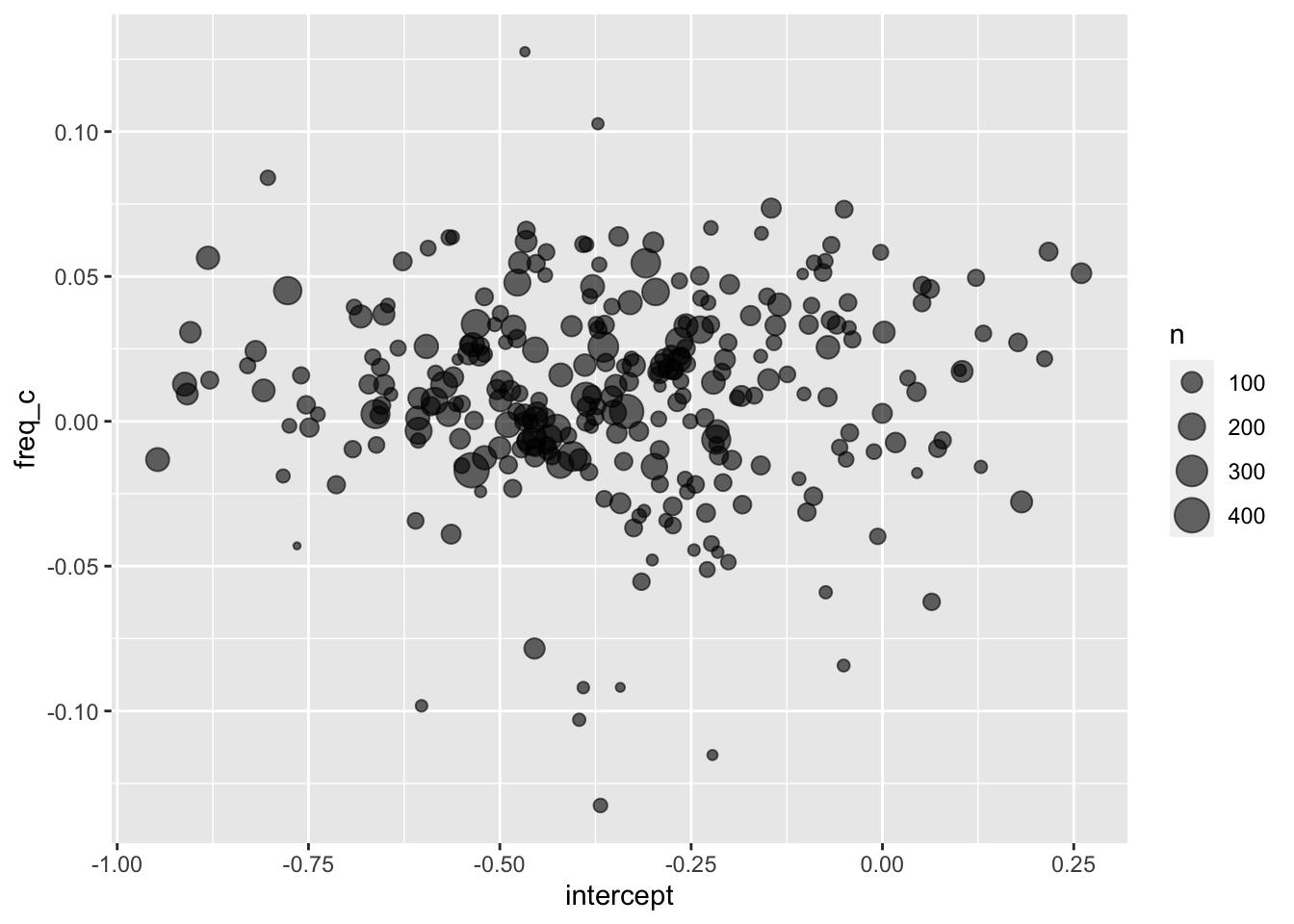
# … with abbreviated variable names ¹​std.error, ²​statistic

Step 2: Select the columns of interest, and pivot wider

ey_nested_params |> 
  mutate(
    n = map_vec(data, nrow)
  ) |> 
  select(speaker, n, term, estimate) |> 
  pivot_wider(
    names_from = term,
    values_from = estimate
  ) |> 
  janitor::clean_names() ->
  ey_speaker_params

head(ey_speaker_params)

# A tibble: 6 × 4
# Groups:   speaker [6]
  speaker       n intercept   freq_c
  <chr>     <int>     <dbl>    <dbl>
1 PH00-1-1-   110   -0.652   0.0370 
2 PH00-1-2-   141   -0.455  -0.00526
3 PH00-1-3-   192   -0.436  -0.00573
4 PH00-1-4-   125   -0.682   0.0362 
5 PH00-1-5-   204   -0.238   0.0316 
6 PH02-1-1-    62   -0.0987 -0.0313 

ey_speaker_params |> 
  ggplot(aes(intercept, freq_c))+
    geom_point(
      aes(size = n),
      alpha = 0.6
    )

Getting predictions

get_pred_tibble <- function(mod, freq_range){
  predictions(
    mod,
    newdata = datagrid(
      freq_c = seq(freq_range[1], freq_range[2], length = 10) 
    )
  ) |> 
    as_tibble()
}

ey_nested_models |> 
  mutate(
    n = map_vec(data, nrow),
    pred = map(models, get_pred_tibble)
  ) |> 
  select(speaker, n, pred) |> 
  unnest(pred)->
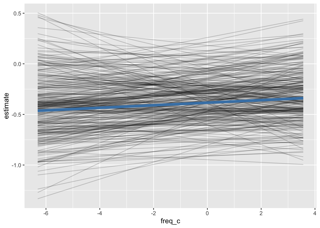
  pred_by_speaker

pred_by_speaker |> 
  ggplot(aes(freq_c, estimate))+
    geom_line(
      aes(group = speaker),
      alpha = 0.2
    )+
    geom_line(
      data = ey_flat_predicted,
      color = "steelblue",
      linewidth = 2
    )

Partial Pooling

a.k.a. mixed effects model.

Specifying and fitting the model

ey_mixed <- lmer(F1_n ~ freq_c + (1 + freq_c | speaker), data = ey_to_model)

summary(ey_mixed)

Linear mixed model fit by REML ['lmerMod']
Formula: F1_n ~ freq_c + (1 + freq_c | speaker)
   Data: ey_to_model

REML criterion at convergence: 30304.5

Scaled residuals: 
     Min       1Q   Median       3Q      Max 
-13.9927  -0.6526  -0.0698   0.5733   8.4810 

Random effects:
 Groups   Name        Variance  Std.Dev. Corr
 speaker  (Intercept) 0.0515319 0.22701      
          freq_c      0.0002979 0.01726  0.01
 Residual             0.2188022 0.46776      
Number of obs: 22269, groups:  speaker, 286

Fixed effects:
             Estimate Std. Error t value
(Intercept) -0.352428   0.014030 -25.120
freq_c       0.011797   0.001658   7.116

Correlation of Fixed Effects:
       (Intr)
freq_c 0.038 

tidy(ey_mixed)

# A tibble: 6 × 6
  effect   group    term                    estimate std.error statistic
  <chr>    <chr>    <chr>                      <dbl>     <dbl>     <dbl>
1 fixed    <NA>     (Intercept)             -0.352     0.0140     -25.1 
2 fixed    <NA>     freq_c                   0.0118    0.00166      7.12
3 ran_pars speaker  sd__(Intercept)          0.227    NA           NA   
4 ran_pars speaker  cor__(Intercept).freq_c  0.00538  NA           NA   
5 ran_pars speaker  sd__freq_c               0.0173   NA           NA   
6 ran_pars Residual sd__Observation          0.468    NA           NA   

Compare to the flat model

tidy(ey_flat)

# A tibble: 2 × 5
  term        estimate std.error statistic  p.value
  <chr>          <dbl>     <dbl>     <dbl>    <dbl>
1 (Intercept)  -0.384    0.00352    -109.  0       
2 freq_c        0.0126   0.00126      10.0 1.60e-23

Comparison to the no-pooling models

ranef(ey_mixed)$speaker |> 
  janitor::clean_names() |>
  rownames_to_column("speaker") |> 
  mutate(
    intercept = intercept + fixef(ey_mixed)[1],
    freq_c = freq_c + fixef(ey_mixed)[2]
  )->
  mixed_speaker_params

mixed_speaker_params |> 
  ggplot(aes(intercept, freq_c))+
    geom_point()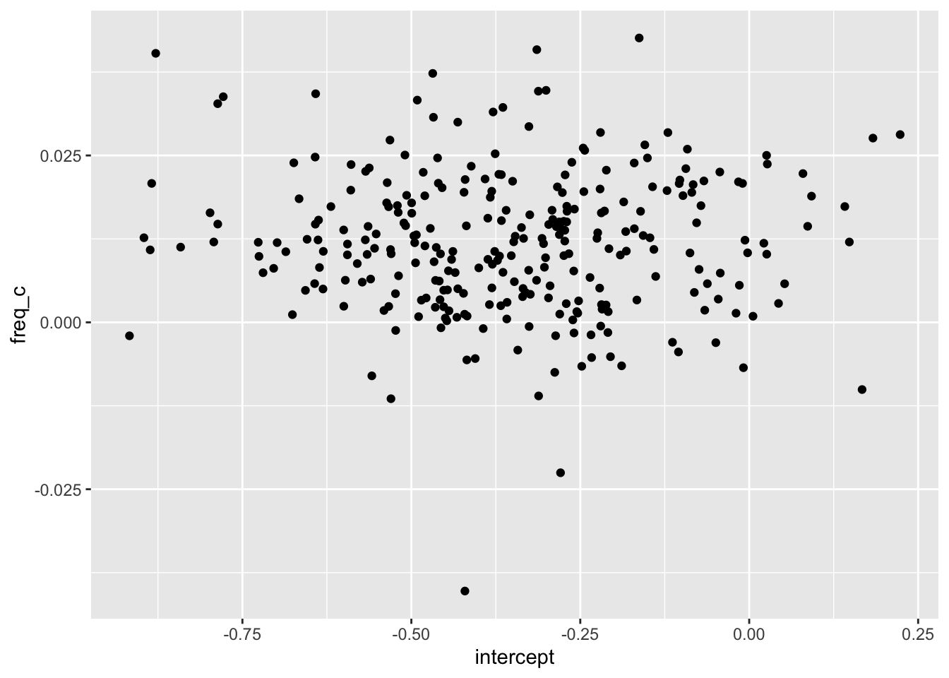

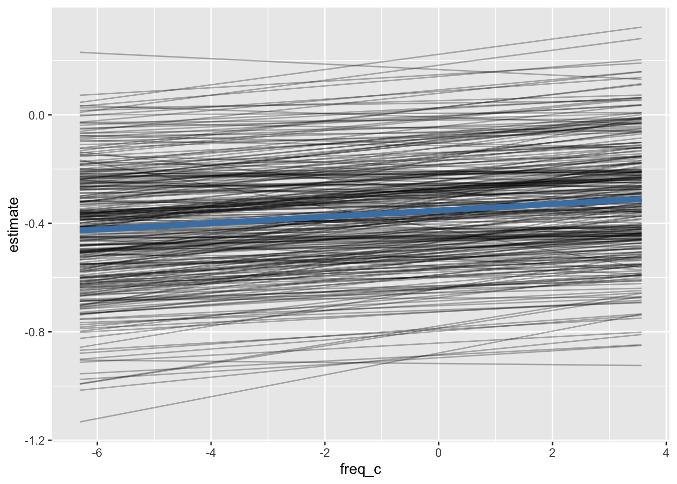
Getting predictions

For each speaker

predictions(
  ey_mixed,
  newdata = datagrid(
    freq_c = seq(freq_range[1], freq_range[2], length = 10),
    speaker = unique(ey_dat$speaker)
  )
) |> 
  as_tibble() ->
  mixed_group_pred

Just the fixed effects.

predictions(
  ey_mixed,
  re.form = NA,
  newdata = datagrid(
    freq_c = seq(freq_range[1], freq_range[2], length = 10)
  )
) |> 
  as_tibble()->
  mixed_fixed_pred

mixed_group_pred |> 
  ggplot(aes(freq_c, estimate))+
    geom_line(
      aes(group = speaker),
      alpha = 0.3
    )+
    geom_line(
      data = mixed_fixed_pred,
      color = "steelblue",
      linewidth = 2
    )

More than one grouping factor

You couldn’t look at both speaker and word grouping effects in the no-pooling approach

ey_mixed2 <- lmer(F1_n ~ freq_c + (1 + freq_c | speaker) + (1 | word), data = ey_to_model)

summary(ey_mixed2)

Linear mixed model fit by REML ['lmerMod']
Formula: F1_n ~ freq_c + (1 + freq_c | speaker) + (1 | word)
   Data: ey_to_model

REML criterion at convergence: 27050.8

Scaled residuals: 
     Min       1Q   Median       3Q      Max 
-15.5631  -0.6201  -0.0521   0.5600   9.6964 

Random effects:
 Groups   Name        Variance  Std.Dev. Corr
 word     (Intercept) 0.0525761 0.2293       
 speaker  (Intercept) 0.0495451 0.2226       
          freq_c      0.0002073 0.0144   0.15
 Residual             0.1819768 0.4266       
Number of obs: 22269, groups:  word, 735; speaker, 286

Fixed effects:
             Estimate Std. Error t value
(Intercept) -0.365703   0.023929 -15.283
freq_c       0.006999   0.004179   1.675

Correlation of Fixed Effects:
       (Intr)
freq_c 0.672 

tidy(ey_mixed2)

# A tibble: 7 × 6
  effect   group    term                    estimate std.error statistic
  <chr>    <chr>    <chr>                      <dbl>     <dbl>     <dbl>
1 fixed    <NA>     (Intercept)             -0.366     0.0239     -15.3 
2 fixed    <NA>     freq_c                   0.00700   0.00418      1.67
3 ran_pars word     sd__(Intercept)          0.229    NA           NA   
4 ran_pars speaker  sd__(Intercept)          0.223    NA           NA   
5 ran_pars speaker  cor__(Intercept).freq_c  0.154    NA           NA   
6 ran_pars speaker  sd__freq_c               0.0144   NA           NA   
7 ran_pars Residual sd__Observation          0.427    NA           NA   

ranef(ey_mixed2)$word |> 
  janitor::clean_names() |> 
  rownames_to_column() |> 
  arrange(intercept) |> 
  head()

      rowname  intercept
1 association -0.4122733
2        gave -0.3925951
3        gate -0.3473580
4       waste -0.3430363
5   radiation -0.3422552
6         hat -0.3366734

Reuse