Distributions

install.packages("droll")

library(droll)
library(tidyverse)

── Attaching packages ─────────────────────────────────────── tidyverse 1.3.2 ──
✔ ggplot2 3.4.0     ✔ purrr   1.0.1
✔ tibble  3.1.8     ✔ dplyr   1.1.0
✔ tidyr   1.3.0     ✔ stringr 1.5.0
✔ readr   2.1.3     ✔ forcats 0.5.2
── Conflicts ────────────────────────────────────────── tidyverse_conflicts() ──
✖ dplyr::filter() masks stats::filter()
✖ dplyr::lag()    masks stats::lag()

theme_set(
  theme_bw()
)

Simulating 100 groups rolling a d6 10 times

set.seed(611)

nsim <- 1000

roll_sims <- 
  tibble(
    sim = seq(1,nsim)
  ) |> 
  ## This will simulate 10 rolls of a d6,
  ## once per simulation.
  mutate(
    rolls = map(
      sim, \(x) rroll(10, d6)
    )
  ) |> 
  ## This counts how many times 1 and 6
  ## came up in each simulation
  mutate(
    one_and_six = map_dbl(
      rolls, \(r)sum(r %in% c(1, 6))
    )
  ) 

roll_sims |> 
  ggplot(aes(one_and_six))+
    stat_bin(binwidth = 1)+
    scale_x_continuous(
      breaks = c(0,5,10)
    )+
    expand_limits(x=c(0,10))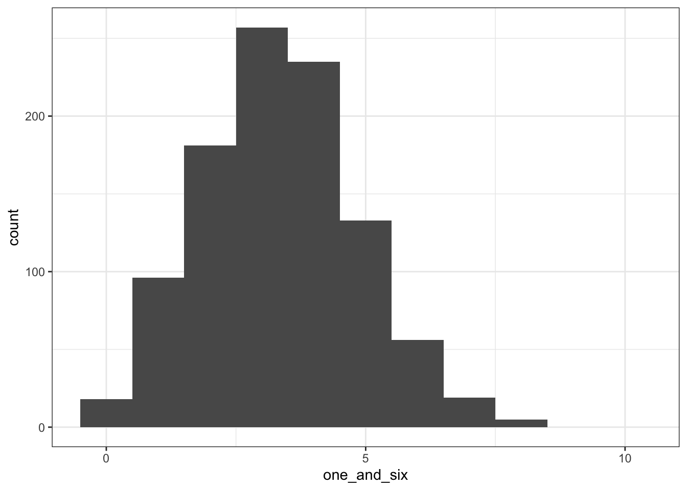

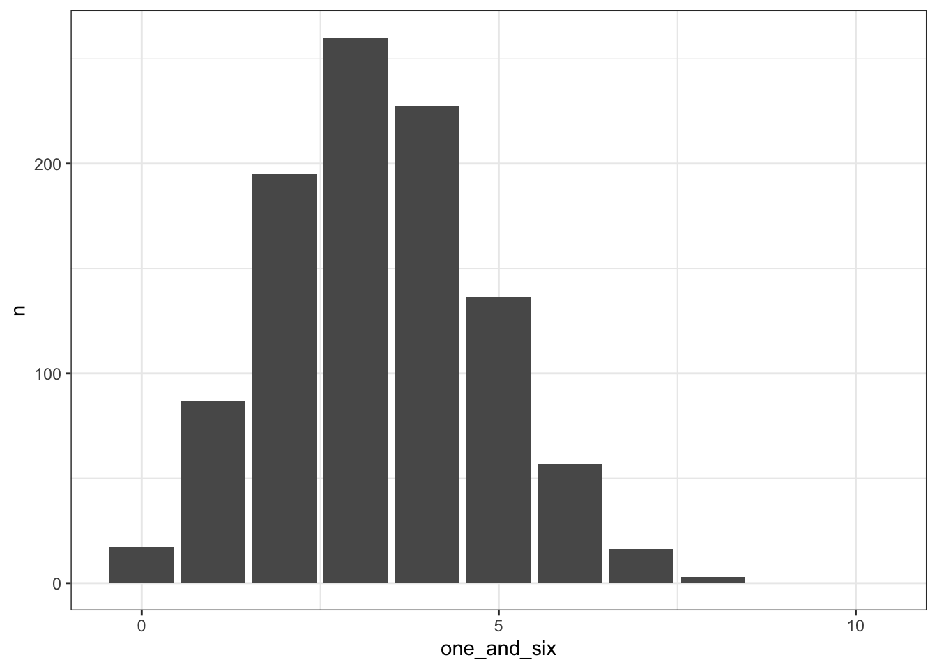
Getting the theoretical distribution

tibble(
  one_and_six = seq(0, 10),
  prob = dbinom(
    one_and_six, 
    size = 10,
    prob = 2/6
  ),
  n = prob * 1000
) |> 
  ggplot(aes(one_and_six, n))+
    geom_col()+
    scale_x_continuous(
      breaks = c(0,5,10)
    )

Reuse