Recap
Grabbing monthly temperature averages for Lexington. Untidy data.
Untidy because each row has 12 different observations (1 for each month). Column names JAN through DEC should be variables.
lex_tempPivoting from wide to long
lex_temp |>
  pivot_longer(
    # which columns should go long?
    cols = JAN:DEC,
    # where should the column names go?
    names_to = "month",
    # where shoild the column values go?
    values_to = "temp"
  )
Getting untidy data
Example untidy (linguistic!) data can be found in Joseph Casillas’ package on github.
install.packages("devtools")
devtools::install_github("jvcasillas/untidydata")library(untidydata)Vowel formant estimates for spanish vowels. The data column label follows good file naming protocol, but poor data column protocol. Three different variables smushed together into one:
speaker id
speaker gender
vowel class
spanish_vowelsThese three columns can be separated out with the tidyr::separate() function.
tidy_vowelsPlotting
Making a ggplot vowel plot from tidy_vowels.
ggplot2 resources
These plots are built by adding “layers”
Data Layer
- The
aes()function is used to map data variables to plot aesthetics.
Geometry layer
“geometries” are the visual components of plots.
tidy_vowels |>
ggplot(aes(x = f2, y = f1)) +
geom_point()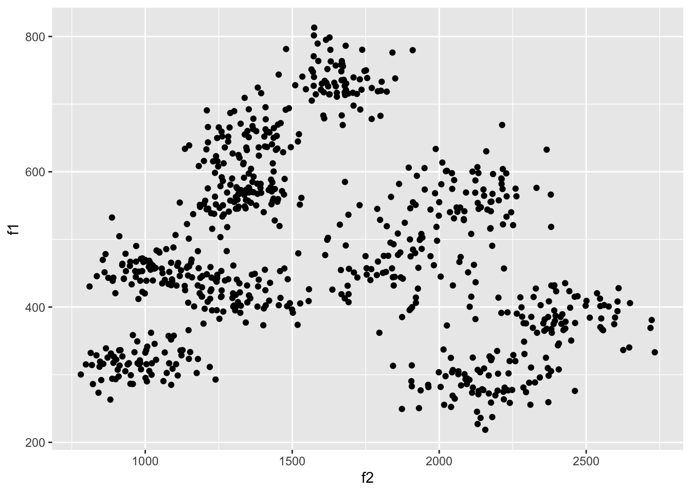
We can set certain visual components of geometries.
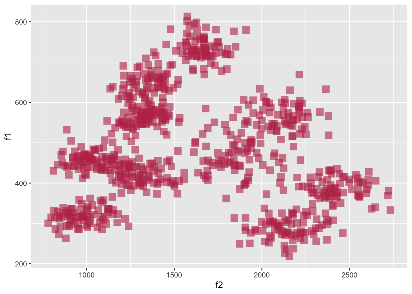
tidy_vowels |>
  ggplot(aes(x = f2, y = f1)) +
    geom_point(
      color = "#BE3455",
      size = 4,
      # alpha is transparency
      alpha = 0.6,
      shape = "square"
    )
We can also map data to the visual components.
tidy_vowels |>
  ggplot(
    aes(
      x = f2,
      y = f1,
      color = vowel
    )
  ) +
    geom_point()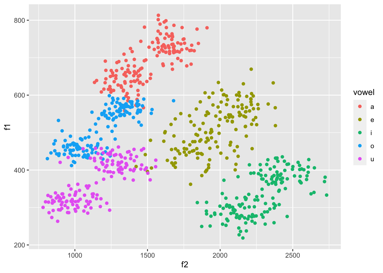
Statistic layers
We can add “statistic” layers to plots as well.
tidy_vowels |>
  ggplot(
    aes(
      x = f2,
      y = f1,
      color = vowel
    )
  ) +
    geom_point()+
    # Doesn't really make sense
    stat_smooth()
`geom_smooth()` using method = 'loess' and formula = 'y ~ x'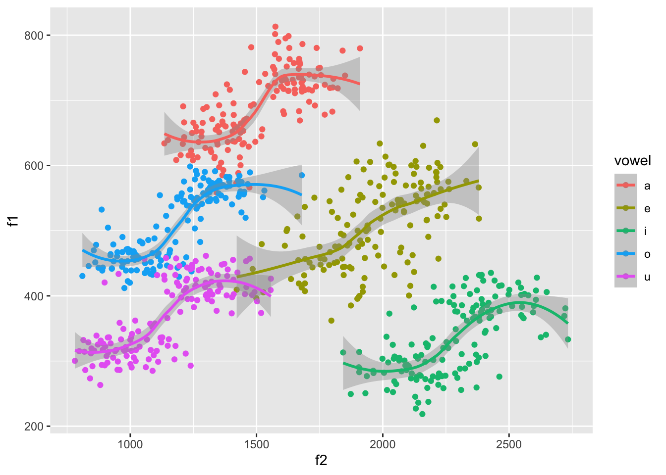
tidy_vowels |>
  ggplot(
    aes(
      x = f2,
      y = f1,
      color = vowel
    )
  ) +
    geom_point()+
    stat_ellipse()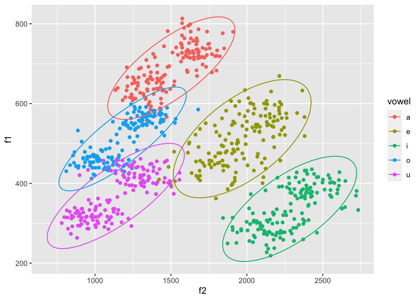
Scale layers
We can adjust the “scales” of the spatial axes and other aesthetic mappings with scale layers.
tidy_vowels |>
  ggplot(
    aes(
      x = f2,
      y = f1,
      color = vowel
    )
  ) +
    geom_point()+
    stat_ellipse()+
    # reverse x and y
    scale_y_continuous(trans = "reverse")+
    scale_x_continuous(trans = "reverse")+
    scale_color_vibrant()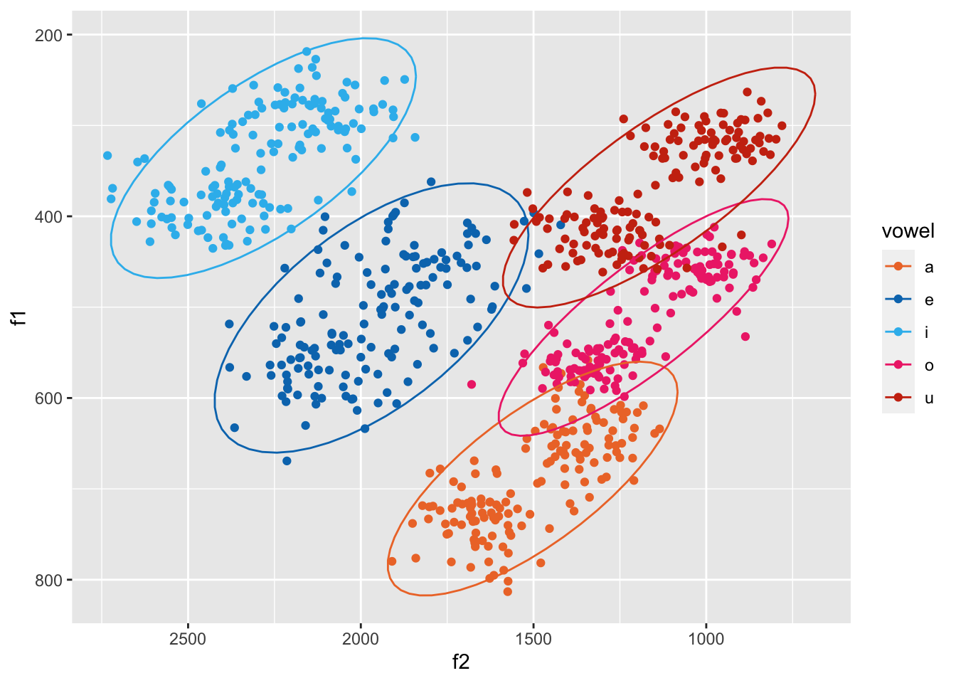
Titles
The ggplot2::labs() layer will do you.
tidy_vowels |>
  ggplot(
    aes(
      x = f2,
      y = f1,
      color = vowel
    )
  ) +
    geom_point()+
    stat_ellipse()+
    # reverse x and y
    scale_y_continuous(trans = "reverse")+
    scale_x_continuous(trans = "reverse")+
    scale_color_vibrant()+
    labs(title = "vowels",
         x = "F2 (hz)",
         y = "F1 (hz)",
         color = "vowel\nclass")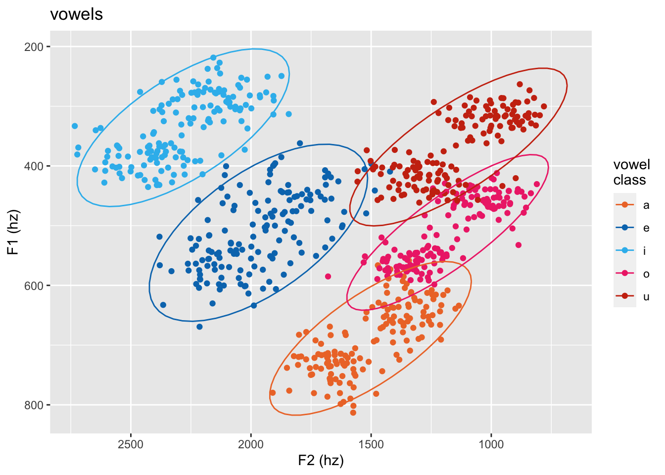
Faceting
You can make small multiples with ggplot2::facet_wrap() or ggplot2::facet_grid().
tidy_vowels |>
ggplot(
aes(
x = f2,
y = f1,
color = vowel
)
) +
geom_point()+
stat_ellipse()+
# reverse x and y
scale_y_continuous(trans = "reverse")+
scale_x_continuous(trans = "reverse")+
scale_color_vibrant()+
labs(title = "vowels",
x = "F2 (hz)",
y = "F1 (hz)",
color = "vowel\nclass")+
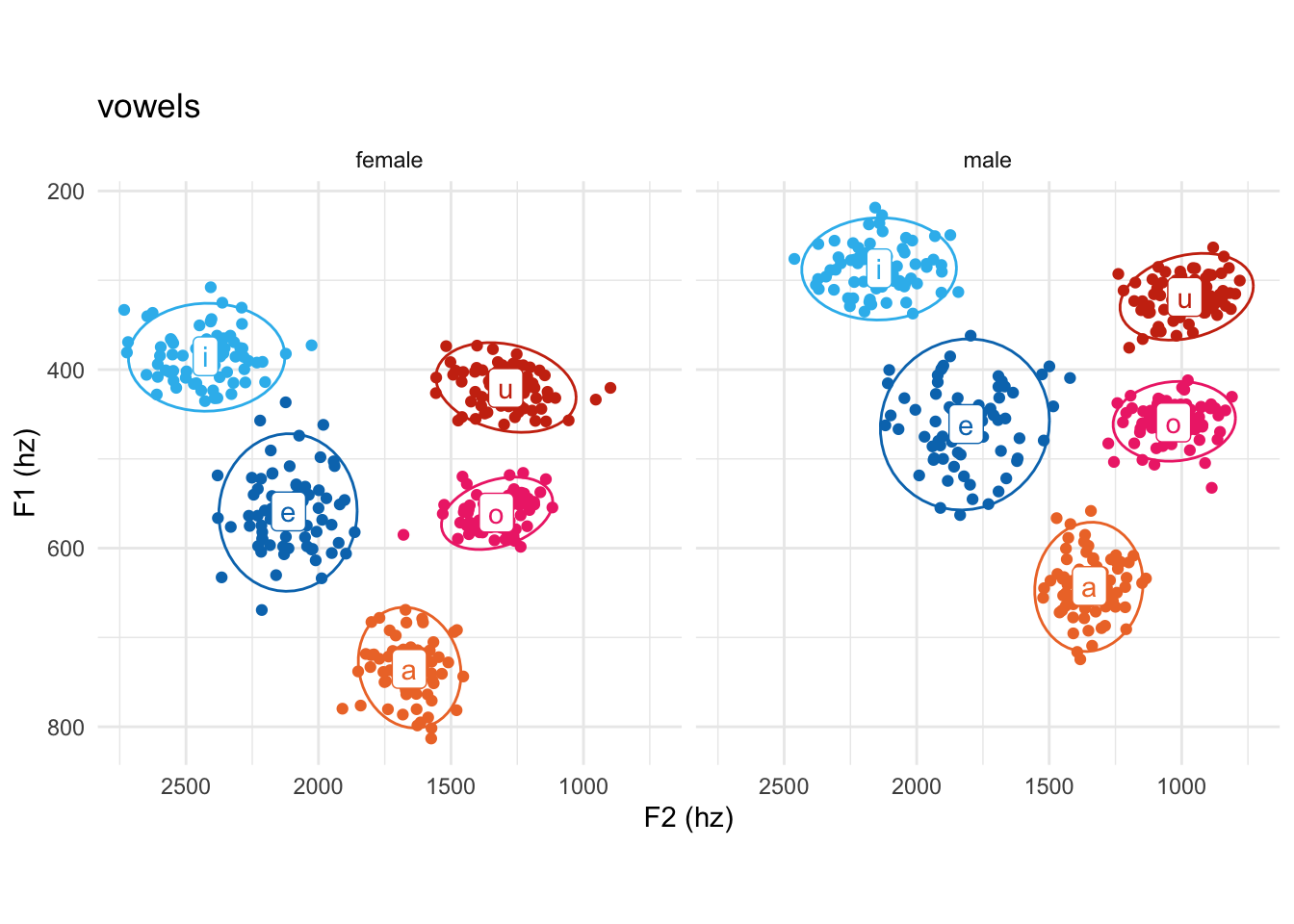
facet_wrap(~gender)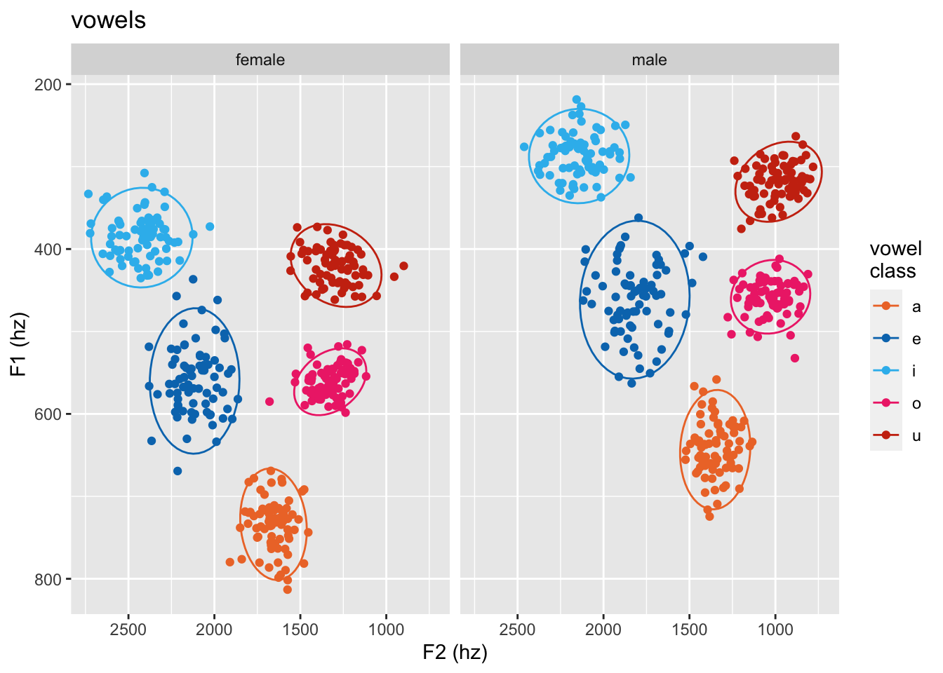
Theming
ggplot2 has a number of built in themes
tidy_vowels |>
  ggplot(
    aes(
      x = f2,
      y = f1,
      color = vowel
    )
  ) +
    geom_point()+
    stat_ellipse()+
    # reverse x and y
    scale_y_continuous(trans = "reverse")+
    scale_x_continuous(trans = "reverse")+
    scale_color_vibrant()+
    labs(title = "vowels",
         x = "F2 (hz)",
         y = "F1 (hz)",
         color = "vowel\nclass")+
    facet_wrap(~gender) +
    theme_minimal()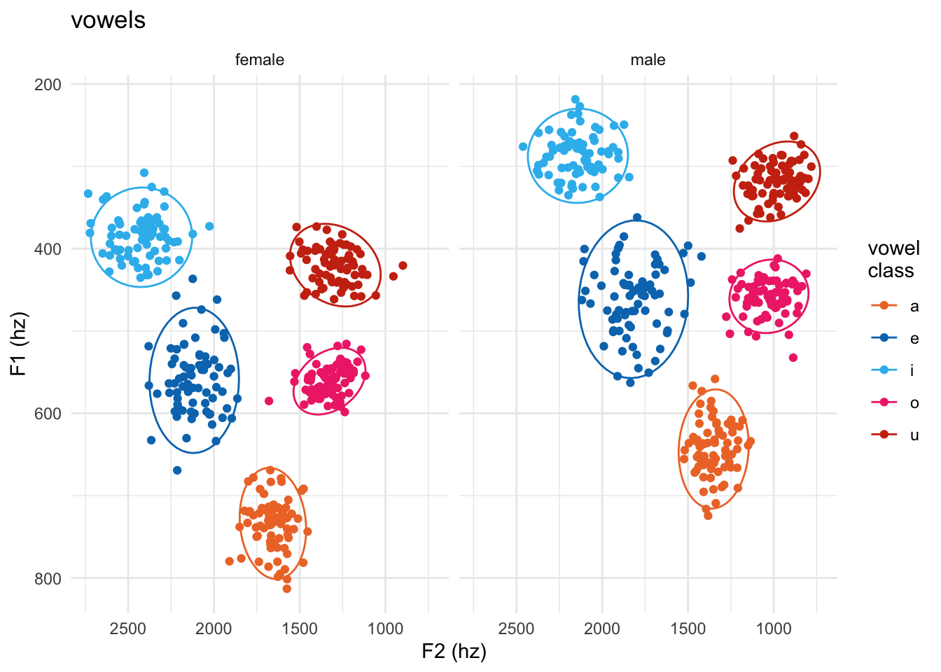
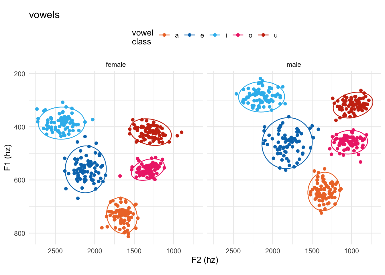
You can get additional fine-grained control with ggplot2::theme()
tidy_vowels |>
  ggplot(
    aes(
      x = f2,
      y = f1,
      color = vowel
    )
  ) +
    geom_point()+
    stat_ellipse()+
    # reverse x and y
    scale_y_continuous(trans = "reverse")+
    scale_x_continuous(trans = "reverse")+
    scale_color_vibrant()+
    labs(title = "vowels",
         x = "F2 (hz)",
         y = "F1 (hz)",
         color = "vowel\nclass")+
    facet_wrap(~gender) +
    theme_minimal() +
    theme(
      legend.position = "top",
      aspect.ratio = 1
      )
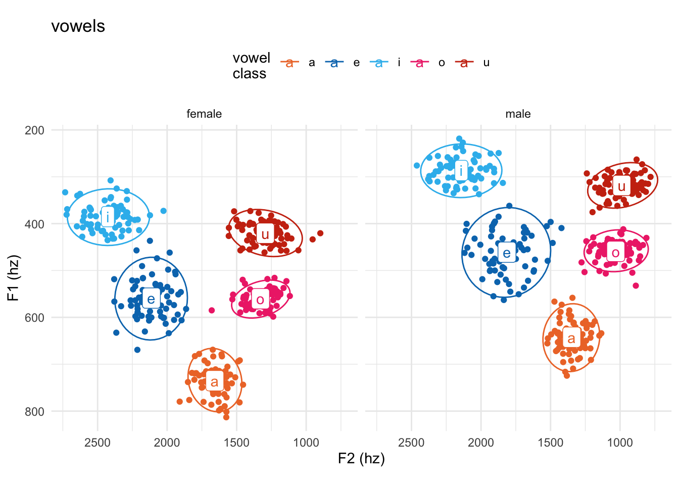
Combining with tidy workflows
To label each vowel cluster with its vowel class, we need to calculate the F1 and F2 means for each vowel for each gender.
`summarise()` has grouped output by 'vowel'. You can override using the
`.groups` argument.
Now add a geom_label() layer on after the geom_point() layer.
tidy_vowels |>
  ggplot(
    aes(
      x = f2,
      y = f1,
      color = vowel
    )
  ) +
    geom_point()+
    geom_label(
      data = vowel_means,
      aes(label = vowel)
    )+
    stat_ellipse()+
    # reverse x and y
    scale_y_continuous(trans = "reverse")+
    scale_x_continuous(trans = "reverse")+
    scale_color_vibrant()+
    labs(title = "vowels",
         x = "F2 (hz)",
         y = "F1 (hz)",
         color = "vowel\nclass")+
    facet_wrap(~gender) +
    theme_minimal() +
    theme(
      legend.position = "top",
      aspect.ratio = 1
      )
Strictly speaking, the legend isn’t necessary anymore with the direct labels. I’ll drop it with the guides() layer. I’ve placed it after the scale_ layers, just for code clarity.
tidy_vowels |>
  ggplot(
    aes(
      x = f2,
      y = f1,
      color = vowel
    )
  ) +
    geom_point()+
    geom_label(
      data = vowel_means,
      aes(label = vowel)
    )+
    stat_ellipse()+
    # reverse x and y
    scale_y_continuous(trans = "reverse")+
    scale_x_continuous(trans = "reverse")+
    scale_color_vibrant()+
    guides(color = "none")+
    labs(title = "vowels",
         x = "F2 (hz)",
         y = "F1 (hz)",
         color = "vowel\nclass")+
    facet_wrap(~gender) +
    theme_minimal() +
    theme(
      aspect.ratio = 1
      )