Starting Multivariate Models

library(tidyverse)
library(broom)
library(marginaleffects)

word_rt <- read_csv("https://raw.githubusercontent.com/bodowinter/applied_statistics_book_data/master/ELP_length_frequency.csv")

Rows: 33075 Columns: 4
── Column specification ────────────────────────────────────────────────────────
Delimiter: ","
chr (1): Word
dbl (3): Log10Freq, length, RT

ℹ Use `spec()` to retrieve the full column specification for this data.
ℹ Specify the column types or set `show_col_types = FALSE` to quiet this message.

Plots

Making plots of the data before we start modelling:

word_rt |>
  ggplot(aes(Log10Freq, RT)) +
    #geom_point()
    stat_bin_2d()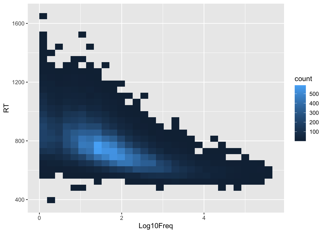

Looks like a negative effect of word frequency on reaction time

word_rt |>
  ggplot(aes(length, RT)) +
    stat_bin_2d()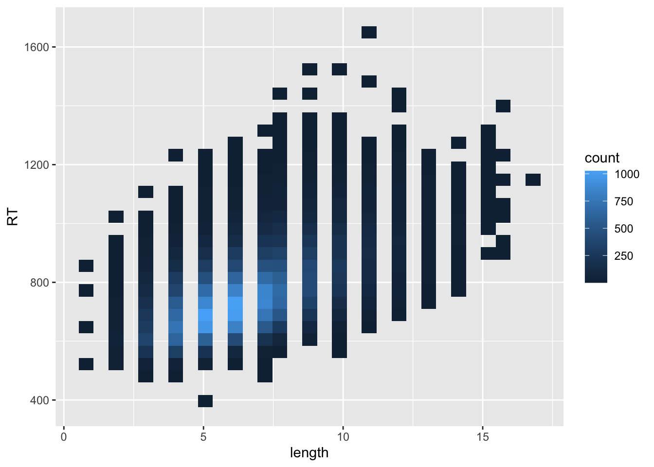

Looks like a positive effect of word length on reaction time.

word_rt |>
  ggplot(aes(Log10Freq, length)) +
    stat_bin_2d()+
    stat_smooth()

`geom_smooth()` using method = 'gam' and formula = 'y ~ s(x, bs = "cs")'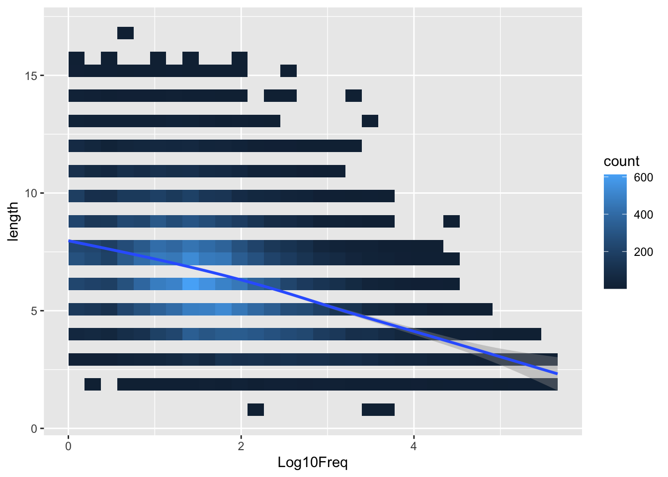

Looks like word frequency and word length are slightly collinear.

Not ideal (modelling without centering and scaling)

lm fits the model.

model_0 <- lm(RT ~ Log10Freq + length, data = word_rt)

tidy(model_0)

# A tibble: 3 × 5
  term        estimate std.error statistic p.value
  <chr>          <dbl>     <dbl>     <dbl>   <dbl>
1 (Intercept)    748.      2.18      344.        0
2 Log10Freq      -68.0     0.594    -115.        0
3 length          19.5     0.238      81.9       0

The (Intercept) value is the predicted value of RT when both Log10Freq and length are 0. Not a likely combination of values.

Goodness of fit:

glance(model_0)

# A tibble: 1 × 12
  r.squared adj.r.sq…¹ sigma stati…² p.value    df  logLik    AIC    BIC devia…³
      <dbl>      <dbl> <dbl>   <dbl>   <dbl> <dbl>   <dbl>  <dbl>  <dbl>   <dbl>
1     0.487      0.487  89.1  15717.       0     2 -1.95e5 3.91e5 3.91e5  2.62e8
# … with 2 more variables: df.residual <int>, nobs <int>, and abbreviated
#   variable names ¹​adj.r.squared, ²​statistic, ³​deviance

Scaling and Centering

We’ll center both predictors on their means, and scale by the standard deviation:

word_rt |>
  mutate(
    log_freq_z = (Log10Freq - mean(Log10Freq))/sd(Log10Freq),
    len_z = (length - mean(length))/sd(length)
  ) ->
  word_rt_scaled

Let’s actually fit three models,

1. One for just frequency
2. One for just length
3. One for frequency and length

model_f <- lm(RT ~ log_freq_z, data = word_rt_scaled)
model_l <- lm(RT ~ len_z, data = word_rt_scaled)
model_fl <- lm(RT ~ len_z + log_freq_z, data = word_rt_scaled)

We can examine all of these models goodness of fits together.

list(
  freq = model_f,
  length = model_l,
  freq_length = model_fl
) |>
  map_dfr(glance, .id = "model") |> 
  select(model, r.squared, adj.r.squared, AIC, BIC)

# A tibble: 3 × 5
  model       r.squared adj.r.squared     AIC     BIC
  <chr>           <dbl>         <dbl>   <dbl>   <dbl>
1 freq            0.383         0.383 396956. 396981.
2 length          0.284         0.284 401905. 401930.
3 freq_length     0.487         0.487 390856. 390889.

The first thing to notice is that even though we’ve centered and scaled the data, the goodness of fit metrics for the freq_length mode, (r-squared and adjusted r-squared) are identical to the original multivariate model.

Also, the goodness of fit always gets better when we add a new predictor, but the adjusted r squared, AIC and BIC try to balance out the complexity of the model and the goodness of fit.

Evaluating the model

We can merge information from the model onto the original data with augment().

augment(model_fl, word_rt_scaled) |>
  ggplot(aes(.fitted, .resid))+
    geom_point()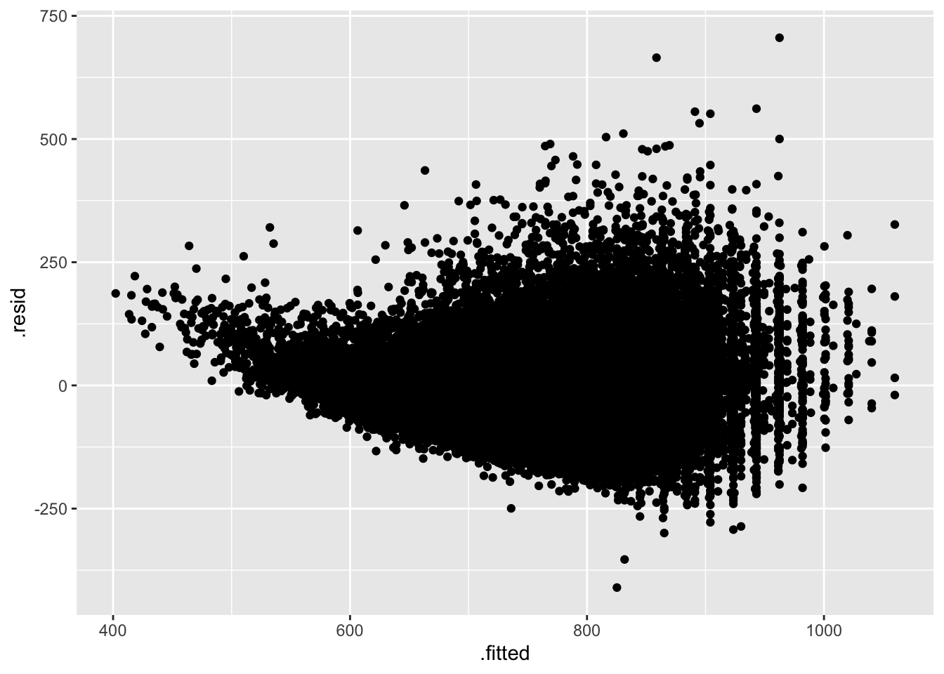

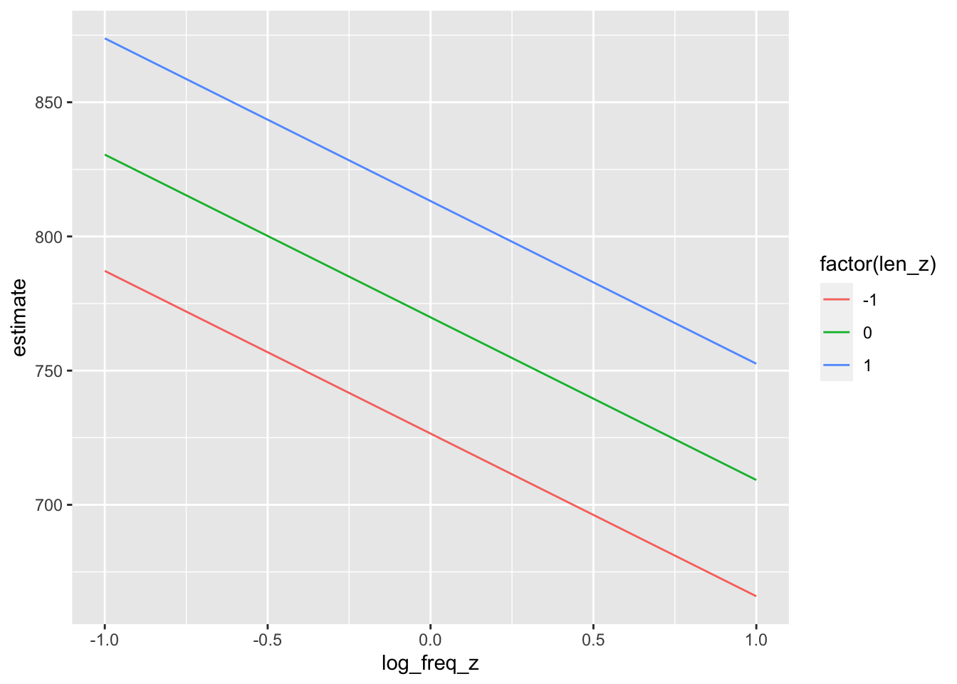
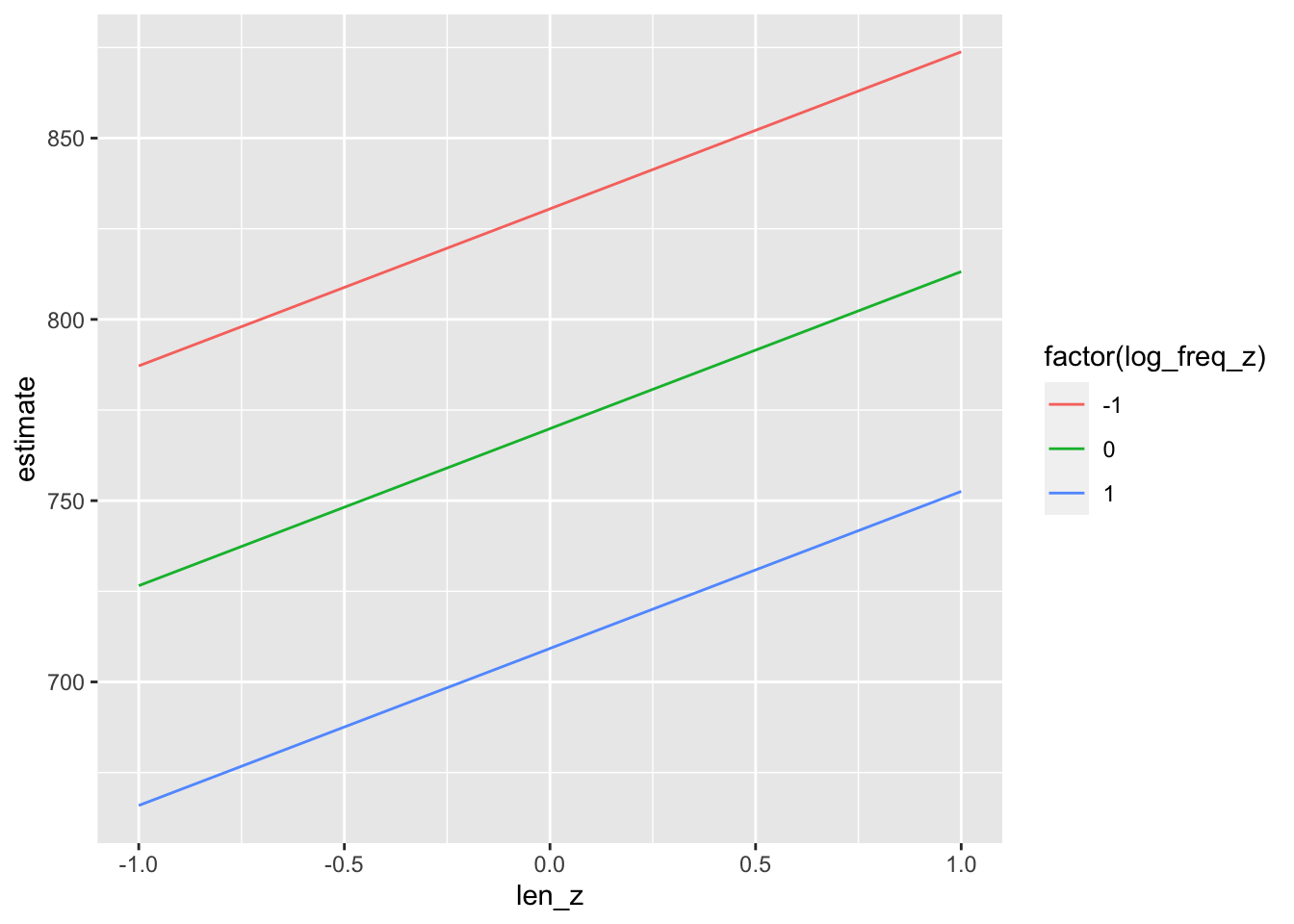
We can also look at the predicted values with marginaleffects::predictions()

predictions(model_fl, 
            newdata = datagrid(log_freq_z = c(-1, 0, 1),
                               len_z = c(-1, 0, 1))) |>
  tibble()->
  predictions_fl

predictions_fl |> 
  ggplot(aes(log_freq_z, estimate))+
    geom_line(aes(color = factor(len_z)))

predictions_fl |> 
  ggplot(aes(len_z, estimate))+
    geom_line(aes(color = factor(log_freq_z)))

Reuse