The Discrete Cosine Transform

library(tidynorm)
library(dplyr)
library(tibble)
library(ggplot2)

plotting defaults

options(
  ggplot2.discrete.colour = c(
    lapply(
      1:6,
      \(x) c(
        "#4477AA", "#EE6677", "#228833",
        "#CCBB44", "#66CCEE", "#AA3377"
      )[1:x]
    )
  ),
  ggplot2.discrete.fill = c(
    lapply(
      1:6,
      \(x) c(
        "#4477AA", "#EE6677", "#228833",
        "#CCBB44", "#66CCEE", "#AA3377"
      )[1:x]
    )
  )
)

theme_set(
  theme_minimal(
    base_size = 16
  )
)

A brief description

The Discrete Cosine Transform re-describes an input signal as a set of coefficients. These coefficients can be converted back into the original signal, or simplified, to get back a smoothed form of the original signal.

For example here is an F1 track with 20 measurement points from the speaker_tracks data set.

one_track <- speaker_tracks |>
  filter(
    speaker == "s01",
    id == 9
  )

one_track |>
  ggplot(aes(t, F1)) +
  geom_point() +
  geom_line()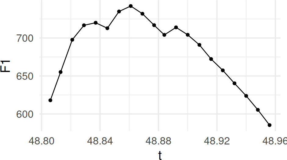

Figure 1: F1 Formant Track

If we apply dct() to the F1 track, we’ll get back 20 DCT coefficients.

dct(one_track$F1)
#>  [1] 482.3728655  16.5472580 -25.0305876  -3.4475760  -8.8201713  -2.4903558
#>  [7]  -3.1619876  -2.9428915  -5.2993291  -0.9811638   0.5681181   0.7707920
#> [13]  -0.4318330   0.2322257  -0.3945702  -0.5995980  -0.4285492   0.8180725
#> [19]   0.7793962  -0.1793681

And, if we apply idct() to these coefficients, we’ll get back the original track.

one_track |>
  mutate(
    F1_dct = dct(F1),
    F1_idct = idct(F1_dct)
  ) |>
  ggplot(
    aes(t, F1_idct)
  ) +
  geom_point() +
  geom_line()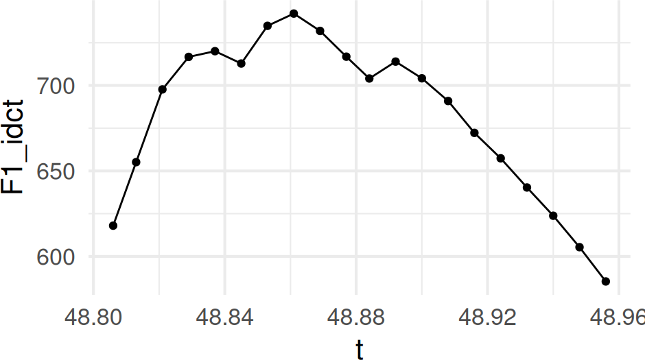

Figure 2: idct(dct(F1))

However, if we apply idct() to just the first few DCT coefficients, we’ll get back a smoothed version of the formant track.

one_track |>
  mutate(
    F1_dct = dct(F1),
    F1_idct = idct(F1_dct[1:5], n = n())
  ) |>
  ggplot(
    aes(t, F1_idct)
  ) +
  geom_point() +
  geom_line()

Figure 3: DCT smoothed F1

DCT functions in tidynorm

There are three reframe_with_* functions in tidynorm.

• reframe_with_dct()

  • This will take a data frame of formant tracks, and return a data frame of DCT coefficients.

  • You need to be able to identify which rows belong to individual tokens, and can identify a column for the time domain.

• reframe_with_idct()

  • This will take a data frame of DCT coefficients, and return a data frame of formant tracks.

  • You need to be able to identify which rows belong to individual tokens, and can identify a column for the parameter number.

• reframe_with_dct_smooth()

  • This combines reframe_with_dct() and reframe_with_idct() into one step, taking in a data frame of formant tracks, and returning a data frame of smoothed formant tracks.

  • You need to be able to identify which rows belong to individual tokens, and can identify a column for the time domain.

Getting average formant tracks

To get average formant tracks for each vowel, you’ll need to

1. Reframe the original formant tracks as DCT coefficients.
2. Average over each parameter number for every vowel.
3. Reframe these averages using the inverse DCT.

# focusing on one speaker
one_speaker <- speaker_tracks |>
  filter(speaker == "s01")

dct_smooths <- one_speaker |>
  # step 1, reframing as dct coefficients
  reframe_with_dct(
    F1:F3,
    .token_id_col = id,
    .time_col = t
  ) |>
  # step 2, averaging over parameter number and vowel
  summarise(
    across(F1:F3, mean),
    .by = c(.param, plt_vclass)
  ) |>
  # step 3, reframing with inverse DCT
  reframe_with_idct(
    F1:F3,
    # this time, the id column is the vowel class
    .token_id_col = plt_vclass,
    .param_col = .param
  )

dct_smooths |>
  filter(
    plt_vclass %in% c("iy", "ey", "ay", "ay0", "oy")
  ) |>
  ggplot(
    aes(F2, F1)
  ) +
  geom_path(
    aes(
      group = plt_vclass,
      color = plt_vclass
    ),
    arrow = arrow()
  ) +
  scale_y_reverse() +
  scale_x_reverse()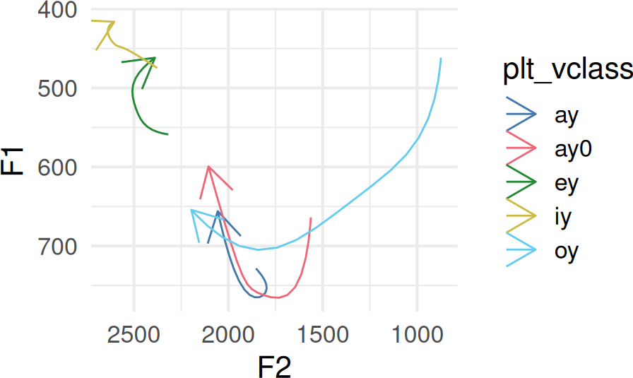

Figure 4: DCT smoothed formant trajectories.

The DCT Basis

The DCT decomposes an input signal as a combination of weighted cosine functions, and returns those weights. You can access the cosine functions it uses with dct_basis().

basis <- dct_basis(100, 5)
matplot(basis, type = "l", lty = 1, lwd = 2)

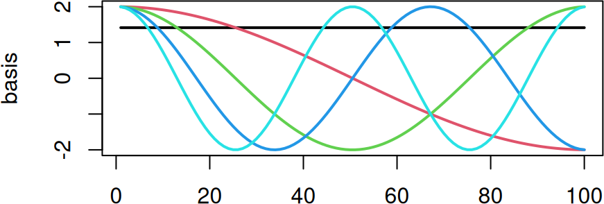
One way to think about it is that the DCT is using these cosine functions in a regression, and the values that get returned are the coefficients.

dct(one_track$F1)[1:5]
#> [1] 482.372866  16.547258 -25.030588  -3.447576  -8.820171

lm(
  one_track$F1 ~ dct_basis(20, 5) - 1
) |>
  coef()
#> dct_basis(20, 5)1 dct_basis(20, 5)2 dct_basis(20, 5)3 dct_basis(20, 5)4 
#>        482.372866         16.547258        -25.030588         -3.447576 
#> dct_basis(20, 5)5 
#>         -8.820171

For more details on the mathematical formulation of the DCT, see the dct() help page.