import numpy as np
def sigmoid(arr):
"""
return the sigmoid, or logit, or softmax transform of an array of numbers
"""
out = np.exp(arr)/(np.exp(arr).sum())
return(out)word2vec
word vectors
Sparse Term-Context Matrix
When we built term-context matrices, the values that went into each cell of the word-by-context matrix were fairly concrete. Let’s look these two example of the word monster as our target word and its surrounding context
['wretch', 'the', 'miserable', 'monster', 'whom', 'i', 'had']
['i', 'was', 'the', 'monster', 'that', 'he', 'said']
With these two windows of context around the target word, we’d go in and fill in the term-context matrix with the counts of every word that appeared in the context of monster. I’m also going to fill in some made up numbers for the word fiend.
grabbed |
the |
wretch |
whom |
had |
that |
he |
was |
i |
said |
lurched |
|
|---|---|---|---|---|---|---|---|---|---|---|---|
| … | |||||||||||
monster |
0 | 2 | 1 | 1 | 1 | 1 | 1 | 1 | 2 | 1 | 0 |
fiend |
1 | 1 | 0 | 0 | 1 | 1 | 2 | 1 | 0 | 0 | 2 |
| … |
With these vectors for monster and fiend we could get a measure of their similarity by taking their dot product (multiplying the values elementwise, then summing up).
monster  0  2  1  1  1  1  1  1  2  1  0
  x
fiend    1  1  0  0  1  1  2  1  0  0  0
  =
         1  2  0  0  1  1  2  1  0  0  0
                       SUM
                        =
                        8
A problem with term-context matrices (that can’t even be solved by converting them to Positive Pointwise Mutual Information) is that they are sparse, mostly filled with 0s. This can be a problem mathematically, since having a lot of 0s in a data set is really inviting a “divide-by-zero” error at some point, but also a problem data-wise. If I had an enormous corpus, made a term-context matrix out of it, and tried emailing it to you, the file size would be really large, but the vast majority of the file size is taken up just by 0.
Getting more abstract, and dense
There are ~7,000 unique vocabulary items in Frankenstein meaning the term-context vector for every word is ~7,000 numbers long. What if instead of using 7,000 numbers to describe a word’s context, we used something smaller, like 300 numbers, none of which are 0, to describe the word’s context.
A prediction task
The way we’ll get to these vectors of numbers is with a prediction task. We’ll give our prediction model a vector associated with a target word, say monster, and then we’ll give it a vector for a word that actually appears in its context, and another that doesn’t.
word: monster = [, , , , …]
context: miserable = [, , , ,…]
distractor: waddle = [, , , , …]
One way to decide which context word is the real context word is by taking the dot product of each with monster. If we’ve got good numbers in our vectors, the real context word should have a larger dot product.
\[ \text{monster} \cdot \text{miserable} > \text{monster} \cdot \text{waddle} \]
Important
I haven’t said yet how we get good numbers into our vectors to make this process possible! If it seems like we’ve skipped a step, it’s because we have, just so that we can talk about the process conceptually.
Note
This kind of prediction task is also called a “skip-gram model.” If we flipped it around and took context words and tried to predict whether or not a target word appeared in the context, that would be called a “Continuous Bag of Words” model, or CBOW.
Dot products to probabilities
The dot product of the target word vector and the possible context word vectors will just be some number. For illustration, I’m going to make some up.
\[ \text{monster} \cdot\text{miserable} = 0.2 \]
\[ \text{monster}\cdot\text{waddle} = -0.5 \]
Since the task we’re doing is a prediction task, we need to convert these numbers into probabilities. I’m going to the trouble of defining the math for how to do this, rather than just leaving it as the “the largest one wins” for a few reasons:
Re-expressing these dot product numbers as probabilities is actually crucial for the training process of getting “good numbers” into our dot products.
People talk about this process a lot, so it’s useful to know what they’re talking about.
The mathematical expression for squeezing an arbitrary vector of numbers, with values that can range between -\(\infty\) and \(\infty\), into a vector of probabilities ranging between 0 and 1 is:
\[ \frac{\exp(x_i)}{\sum_{i=1}^n\exp(x_i)} \]
This formula has a bunch of different names. In fact, several subfields of linguistics use this formula, and I don’t think they all realize they’re talking about the same thing. Some things this formula can be called:
When there’s just 2 values being converted:
“Sigmoid”, often abbreviated as \(\sigma\) or \(\sigma(x_i)\)
the “logistic transform”, which is the math at the heart of “logistic regression” aka “Varbrul”
When there are multiple values being converted:
“Softmax”, also sometimes abbreviated as \(\sigma\) or \(\sigma(x_i)\)
It’s the formula at the heart of “multinomial regression”
It’s also the formula for Maximum Entropy models, a.k.a. “MaxEnt Grammars” (Hayes and Wilson 2008)
Here’s how to write it out as a python function, using numpy.
dists = np.array([0.2, -0.5])
probs = sigmoid(dists)
print(probs)
[0.66818777 0.33181223]The results
As SLP point out, we actually need two vectors for each word. One for its use as the target word, and one for its behavior as a context word.
monster_tmonster_c
Apparently some approaches will just add together these two vectors elementwise, and others will throw away the context vectors.
Either way, assuming we’ve gotten some good numbers into these vectors, let’s think about what has been encoded into them. Let’s take two word that are probably very interchangeable in Frankenstein, and two words that probably aren’t.
interchangeable:
monsteranddæmonnot interchangeable:
monsterandcalled
If monster and dæmon are very interchangeable in the text, that means they should have many of the same words in their contexts. That means that for some context word vector, \(c\), we should expect \(\text{monster}\cdot c\) to have a roughly similar result as \(\text{dæmon} \cdot c\), since they’re going to give roughly the same probability to \(c\) being in their context. The only way for that to really happen is if the values in both of their vectors are also very similar to each other.
On the other hand, monster and called aren’t very interchangeable, meaning they don’t have many shared words in their contexts. So for some context word vector \(c\), the dot products \(\text{monster}\cdot c\) and \(\text{called} \cdot c\) should be pretty different, since these two words should make different predictions for the words that appear in their context. And the only way for that to happen is for the values in their vectors to be pretty different from each other.
So, what winds up happening is the word vectors for monster, dæmon and called encode information about the words they appear around, and with that information we can also calculate the cosine similarities between each of them. In that sense, it’s really similar to the term-context counts we were working with before, but now with much smaller vectors (300 numbers instead thousands) and without a lot of zeros.
How it’s done
The way we get good numbers into our word vectors is by starting out with random numbers. Let’s say we started out with this window of words around monster
['wretch', 'the', 'miserable', 'monster', 'whom', 'i', 'had']And we told the prediction model to figure out which of the following words were in the context:
wretchgreenlurched
The model is actually initialized with random values for the target word vector \(\text{monster}_t\) and the context vectors \(\text{wretch}_c\), \(\text{green} _c\) and \(\text{lurched}_c\). So even though we were hoping for a vector like \([1, 0, 0]\) for these three words (1 meaning “is a context word” and 0 meaning “is not a context word”), we might get back a vector (after doing dot-products and the softmax transformation) like \([0.25, 0.30, 0.45]\).
So, that’s a bad result, but the good news is we can calculate exactly how bad with a “loss function.” We already talked a little bit about one kind of loss function, the Mean Squared Error. For a categorical decision like this, the loss function is called “Cross Entropy” and is calculate like so:
Take the log of the predicted probabilities,
Multiply them elementwise by the expected outcomes (zeros and a 1)
Sum them all together
multiply by -1
Here’s how that goes for the illustrative numbers:
Expected:          [  1,     0,     0    ]
    x
log(Prediction:)   [ -1.39, -1.20, -0.79 ]
    =
                   [ -1.39,  0,     0    ]
                             SUM
                             -1.39
                             NEGATIVE
                             1.39
Another way we can express elementwise multiplication and summing would be as a dot product. So, where \(L_{CE}\) stands for “Cross Entropy Loss”, \(y\) is the expected outputs, and \(p\) is the probabilities from the model
\[ L_{CE} = -(y\cdot \log(p)) \]
The way the Cross Entropy Loss relates to probabilities can be visualized like this:
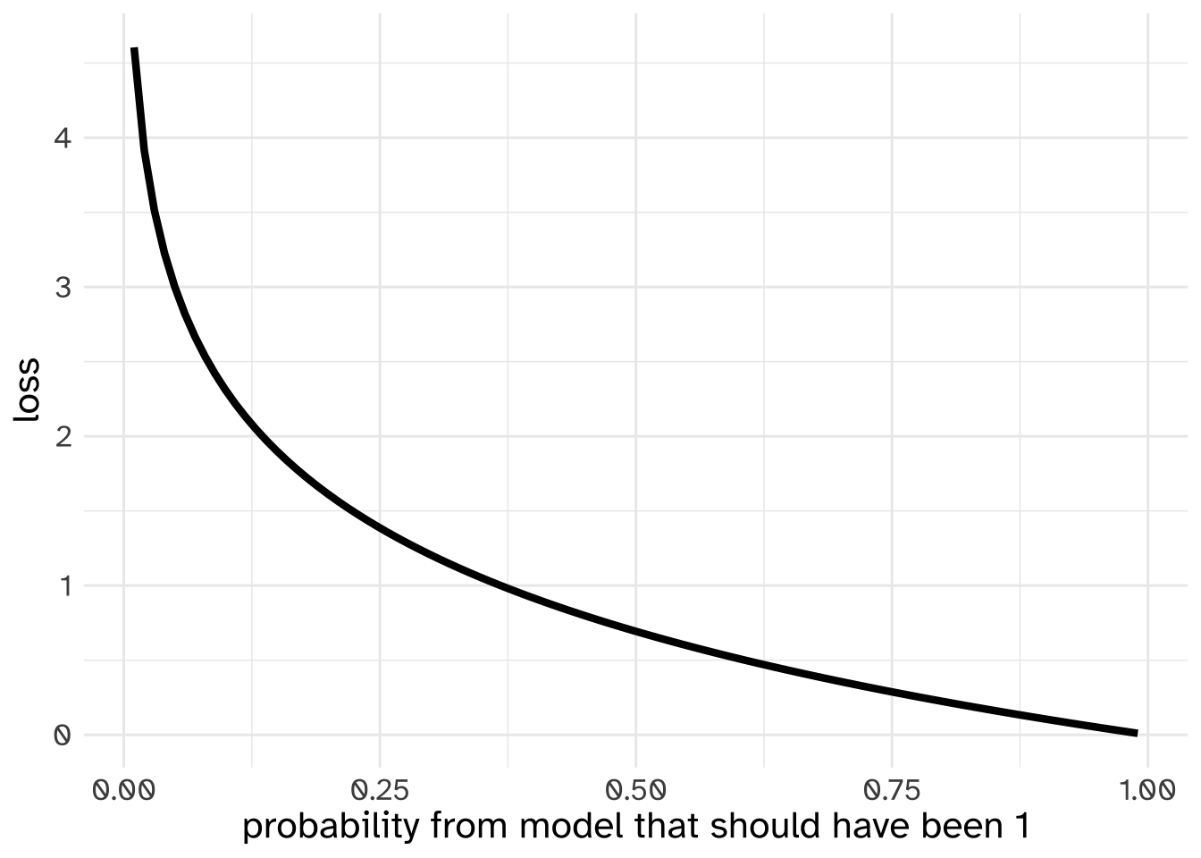
While being able to quantify how bad the prediction was might not seem all that useful in itself, once you have a simple function like this, you can also calculate how much and in which direction you should change the values in your vectors. The math behind that process is a bit beyond the scope of this course, but the process is called “Gradient Decent”, and when used in training neural networks is called “backpropagation.”
What we can do with it.
One thing we can be sure of is that we can’t look at the numbers in these word vectors and find some column that corresponds to a semantic feature we understand. But we can find some patterns in them that seem to correspond to the word’s meaning.
For example, let’s download a pre-trained word vector model1 using the gensim package.
import gensim.downloader as api
wv = api.load('glove-wiki-gigaword-100')
We can get the word vectors for any word that appears in the model’s vocabulary.
print(wv["linguistics"])[ 0.40662 0.459 0.080326 0.64767 0.63911 -0.28373 0.26237
-0.9772 -0.20358 0.54826 -1.1537 -0.50849 0.27668 0.83333
0.11316 0.52335 -0.17736 0.19002 -0.17361 -0.23783 -0.63136
0.45049 0.60977 0.1982 0.22974 -0.68825 0.25491 -0.933
-0.17222 -0.55944 -1.4325 0.32381 -1.0433 -0.27245 -0.66088
0.035583 -0.72584 0.3761 -0.23195 0.050886 -0.86028 -0.43717
-0.8794 -0.037928 -0.69986 0.10677 0.90005 0.26923 -0.36821
0.98975 0.84426 -0.025086 0.47444 -0.31434 -0.31343 0.34649
-0.043019 -1.0718 0.14563 0.45778 0.069034 0.49238 -0.39944
-0.664 0.44024 -0.055936 0.16554 0.1716 0.81233 1.0646
-0.38757 1.3677 0.56161 -0.27431 -0.77989 -0.28478 -0.11712
0.88058 -0.33901 -0.15304 -0.78882 -0.46359 -0.56632 -0.03353
-0.79085 0.97591 -0.005715 -0.25515 0.060361 -0.48979 0.11511
-0.12553 0.10717 0.58306 1.065 0.015627 -0.31298 -0.69456
0.059494 0.51897 ]And we can find words in the model that are most similar to a key word.
from tabulate import tabulate
print(tabulate(wv.most_similar("linguistics")))| anthropology | 0.819153 |
| sociology | 0.763624 |
| philology | 0.758713 |
| mathematics | 0.711027 |
| comparative | 0.700243 |
| biology | 0.698893 |
| zoology | 0.698872 |
| psychology | 0.695841 |
| neuroscience | 0.688815 |
| philosophy | 0.661165 |
What people have also found is that you can do analogies with word vectors. To demonstrate, let’s grab the word vectors for u.k., its capital, london, and france.
uk_vec = wv["u.k."]
london_vec = wv["london"]
france_vec = wv["france"]
We haven’t pulled out the vector for France’s capital, france, but if word meaning has been successfully encoded in these vectors, then the angle (in the huge 100 dimensional space) between london and u.k. should be about the same as it is between france and its capital. Another way to think about it would be to say if we subtracted the u.k. meaning from london, we’d be left with a vector that encodes something about “capitalness” in it. And if we added that to france, we might wind up with a vector that points to a location close to France’s capital!
capitalness_vec = london_vec - uk_vec
france_capital = france_vec + capitalness_vec
print(tabulate(wv.most_similar(france_capital)))| paris | 0.849697 |
| france | 0.791088 |
| london | 0.763334 |
| prohertrib | 0.725074 |
| rome | 0.677958 |
| britain | 0.669977 |
| french | 0.656768 |
| lyon | 0.634014 |
| took | 0.629788 |
| later | 0.623878 |
Visualizing
In order to visualize data from the word vectors, we need to do some “dimensionality reduction” (a topic for another lecture). Bit here’s some basic code to do it.
First, I want to populate a list of words that are all kind of related to each other, which this function ought to do.
Note
This is a “recursive” function. The argument size controlls how many similar words you pull out, and depth controls how many times you try to pull out similar words to those vectors. If you want to figure out how many iterations the function could be going through it’s size ** depth or \(\text{size}^\text{depth}\). So be careful when setting your depth argument too high!
The vocabulary that eventually gets returned won’t be as large as size ** depth, though, since it’s only going to include words once, and words in similar areas of the vector space will probably appear in each other’s searches.
def get_network(wv, words, vocab = set(), size = 10, depth = 2):
  """
    from a list of seed words, get a network of words
  """
  vocab = vocab.union(set(words))
  if depth == 0:
    return(vocab)
  else:
    for w in words:
      sims = wv.most_similar(w, topn = size)
      sim_word = [s[0] for s in sims if not s in vocab]
      vocab = vocab.union(set(sim_word))
      vocab = get_network(wv, sim_word, vocab = vocab, size = size, depth = depth-1)
  return(vocab)
I’ll grab a bunch of words with the starting point of “linguistics.”
ling_similar = get_network(wv,
                            words = ["linguistics"],
                            vocab = set(),
                            size = 10,
                            depth = 4)
After grabbing this set of words, I’ll get their word vectors, and convert them to an array.
lingsim_v = [wv[word] for word in ling_similar]
lingsim_v = np.array(lingsim_v)
At this point, I have to apologize for not knowing how to make graphs in python, and I don’t want to confuse matters by starting to write R code. What you see here is my best attempts after googling, and making graphs with plotly with just the default settings.
#importing plotly
import plotly.express as px
One way we can plot the big matrix of values we have is as a “heatmap” or “image”. In this figure, the x axis represents each word, the y axis represents the positions in the word vectors, and the colors represent the values in the word vectors.
fig = px.imshow(lingsim_v.T)
fig.show()
While that is pretty, it’s not all that informative about what information is represented in the data. And we can’t really make a 100 dimensional plot either. Instead, we need to do boil down these 100 dimensions into 3 or 3 that we can plot. Principle Components Analysis (PCA) is one method that will work, but a popular method for word embeddings and neural networks specifically is t-SNE.2 Here’s how to do t-SNE on our “linguistics” matrix:
from sklearn.manifold import TSNE# the `perplexity` argument affects how "clumpy"
# the result is. Larger numbers have less clumpyness
tsne = TSNE(n_components=2, perplexity = 5)
projections = tsne.fit_transform(lingsim_v)fig = px.scatter(
projections,
# 0 and 1 refer to the columns of
# projections
x=0, y=1,
# I wanted just text, no points
# so I created an array of 0s the same length
# as the number of words
size = np.zeros(len(ling_similar)),
# plot the text of each word.
text = list(ling_similar),
width=800, height=800
)
fig.show()Training our own word2vec models
We can train our own word2vec models using gensim. We need to feed it a list of lists. Something like:
[['i', 'spoke', 'to', 'the', 'monster'],
 ['he', 'looked', 'at', 'me', 'strangely']]
To get this list of list data, I’ll import some of our good tokenizer friends from nltk, and also this time remove stopwords from the data.
from gensim.models import Word2Vec
from nltk.tokenize import sent_tokenize, RegexpTokenizer
from nltk.corpus import stopwords
from pprint import pprint
with open ("gen/books/shelley/84.txt", 'r') as f:
text = f.read()
text = text.replace("\n", " ").lower()
sentences = sent_tokenize(text)
sent_word = [RegexpTokenizer(r"\w+").tokenize(sent) for sent in sentences]
corpus = [[w for w in sent if not w in stopwords.words('english')] for sent in sent_word]
pprint(corpus[10:12])[['productions',
'features',
'may',
'without',
'example',
'phenomena',
'heavenly',
'bodies',
'undoubtedly',
'undiscovered',
'solitudes'],
['may', 'expected', 'country', 'eternal', 'light']]I’ll set a relatively word vector size (100) and pretty narrow window (2 words to each side) and train for a good number of epochs (100).
model = Word2Vec(sentences = corpus,
                 vector_size = 100,
                 window = 2,
                 epochs = 100)
Here’s a table of the most similar words to “monster” in the novel.
print(
  tabulate(
    model.wv.most_similar("monster")
  )
)| hellish | 0.56288 |
| fingers | 0.526299 |
| gigantic | 0.488169 |
| lifeless | 0.479828 |
| filthy | 0.474239 |
| wickedness | 0.471034 |
| shuddered | 0.460071 |
| face | 0.45477 |
| rage | 0.453865 |
| imagined | 0.449275 |
This model has a lot fewer words in it than the big GloVE model we downloaded above, so we can get all of the word vectors as a matrix and plot the t-SNE of the whole book.
frank_matrix = model.wv.get_normed_vectors()frank_matrix.shape(1719, 100)tsne = TSNE(n_components=2, perplexity = 5)
projections = tsne.fit_transform(frank_matrix)vocab = model.wv.index_to_keyfig = px.scatter(
projections,
x=0, y=1,
hover_name = np.array(vocab),
width=800,
height=800
)
fig.show()References
Hayes, Bruce, and Colin Wilson. 2008. “A Maximum Entropy Model of Phonotactics and Phonotactic Learning.” Linguistic Inquiry 39 (3): 379–440. https://doi.org/10.1162/ling.2008.39.3.379.