import numpy as np
import pandas as pd
from palmerpenguins import load_penguins
from sklearn.linear_model import LinearRegression
from sklearn.metrics import mean_squared_error
penguins = load_penguins()Neural Nets
Neural Networks
What are Neural Networks?
The thing we’re going to be talking about in this lecture has had many names over the years, including
Parallel Distributed Processing
Connectionism
Artificial Neural Networks
Neural Networks
Deep Learning
Deep Neural Networks
AI
The basic idea is that we can re-weight and combine input data into a new array of features that can be used as predictors if output values.
The relationship between neural nets and regression
Let’s look at how a linear regression works one more time before we get into neural networks.
penguin_body = penguins.dropna()[
                  ["bill_length_mm",
                   "bill_depth_mm",
                   "flipper_length_mm",
                   "body_mass_g"]]
penguin_body.head()
bill_length_mm bill_depth_mm flipper_length_mm body_mass_g
0 39.1 18.7 181.0 3750.0
1 39.5 17.4 186.0 3800.0
2 40.3 18.0 195.0 3250.0
4 36.7 19.3 193.0 3450.0
5 39.3 20.6 190.0 3650.0Let’s say I wanted to use the bill measurements and flipper measurements to predict the penguin’s body mass. We can do this with a “linear regression.” The linear regression will give us:
An array of numbers we need to multiply each body measurement by and sum up
A constant value to add to the result
And the resulting number will be as close as we can get possible to the actual body mass of the penguin. The way it figures out the best numbers to multiply each body measurement by, and the constant value to add, is by comparing the results we get from that operation to the observed penguin body weight, and minimizing a loss function (mean squared error).
lm = LinearRegression()
X = penguin_body[["bill_length_mm",
                   "bill_depth_mm",
                   "flipper_length_mm"]]
y = penguin_body["body_mass_g"]
linmodel = lm.fit(X, y)linmodel.coef_array([ 3.29286254, 17.83639105, 50.76213167])linmodel.intercept_-6445.476043030191mean_squared_error(linmodel.predict(X), y)152597.3327433967We can get the predicted body mass of the first penguin by doing matrix multiplication and adding in the constant.
(np.array(X)[0, :] @ linmodel.coef_) + linmodel.intercept_3204.761227286078And if we compare this to the actual penguin’s body mass, it’s not too far off!
y[0]3750.0Diagramming the model
We can visualize this regression model with a nodes and arrows figure like this:
These numbers from the model have the benefit of being interpretable. For example, every 1 millimeter a penguin’s bill length gets, we expect its body mass to also increase by 3.29 grams. If we had one reference penguin, and found another one that’s bill was 2 mm longer, but with flippers 1 mm shorter, we would expect its body mass to be (2*3.29) + (-1 * 50.76) = -44.18 grams less.
Combining features
But what if the relationships between input data and output measurements was more complicated? Maybe the two separate bill measurements ought to be combined into one, more holistic “bill size” measurement first.
And maybe we should have a “length of things” combined measure, and combine bill length and flipper length variable also.
If we then used these synthetic variables in our model, it would now look like this:
This is now a kind of “neural network” model. In practice, the synthetic variables are not hand crafted like this. Instead, people set up a “hidden layer” with a set number of “nodes”, and then those nodes get fully connected to all of the inputs. No one knows how the input nodes are supposed to be synthesized into new variables, they just let the model fitting optimize for it.

Building a neural net classifier
In the next few steps, we’ll build up a neural net classifier, and walk through the kind of decisions that are commonly made in constructing these models.
The Data
We’ll be working with vowel formant data, the following code blocks
- Load
pandas, which will read in the data (the output of FAVE-extract on speaker s03 from the Buckeye corpus). - Load
plotly, which I’ll use for making graphs - Reads in the data
- Makes a plot
# Loads libraries
import pandas as pd
import plotly.express as px
# reads in the tab delimited data
vowels = pd.read_csv("data/s03.txt", sep = "\t")
vowels = vowels[["plt_vclass", "ipa_vclass", "word", "F1", "F2", "F3", "dur"]].dropna()# makes an F1 by F2 plot
fig1 = px.scatter(vowels,
x = "F2",
y = "F1",
color = "ipa_vclass",
hover_data = ["word"])
foo = fig1.update_xaxes(autorange = "reversed")
foo = fig1.update_yaxes(autorange = "reversed")
fig1.show()To keep things simpler, let’s try building a classifier that tries to identify which front vowel we’re looking at. Here’s how each vowel category appears in the dataset, along with its lexical set label, just to clear what vowels we’re looking at/
plt_vclass |
ipa_vclass |
Lexical Set |
|---|---|---|
| iy | i | Fleece |
| i | ɪ | Kit |
| ey | ej | Face |
| e | ɛ | Face |
| ae | æ | Trap |
front_tf = vowels["plt_vclass"].isin(["iy", "i", "ey", "e", "ae"])
front_vowels = vowels[front_tf]
Why a Neural Network?
One of the ideas behind a neural network model is that while these 5 categories may each be overlapping on each individual dimension, maybe through some combination of dimensions, they might be separable.
Code
hist_f1 = px.histogram(front_vowels,
                       x = "F1",
                       color = "plt_vclass",
                       marginal = "violin",
                       category_orders={"plt_vclass": ["iy", "i", "ey", "e", "ae"]},
                       title = "Vowels, along F1")
hist_f1.show()
Code
hist_f2 = px.histogram(front_vowels,
                       x = "F2",
                       color = "plt_vclass",
                       marginal = "violin",
                       category_orders={"plt_vclass": ["iy", "i", "ey", "e", "ae"]},
                       title = "Vowels, along F2")
hist_f2.show()
Code
hist_f3 = px.histogram(front_vowels,
                       x = "F3",
                       color = "plt_vclass",
                       marginal = "violin",
                       category_orders={"plt_vclass": ["iy", "i", "ey", "e", "ae"]},
                       title = "Vowels, along F3")
hist_f3.show()
Code
hist_dur = px.histogram(front_vowels,
                       x = "dur",
                       color = "plt_vclass",
                       marginal = "violin",
                       category_orders={"plt_vclass": ["iy", "i", "ey", "e", "ae"]},
                       title = "Vowels, along duration")
hist_dur.show()
Data Preparation
Before trying to train a neural network model, it’s common to “scale” or “normalize” the data. Just the formant data themselves have different ranges they cover, but the duration is on a much smaller scale.
front_vowels.agg(
  {"F1" : ["min", "mean", "max", "std"],
   "F2" : ["min", "mean", "max", "std"],
   "F3" : ["min", "mean", "max", "std"],
   "dur" : ["min", "mean", "max", "std"]}
)
F1 F2 F3 dur
min 213.500000 754.800000 1473.300000 0.050000
mean 471.265951 1679.375168 2550.123948 0.121439
max 949.400000 2646.900000 4362.500000 0.580000
std 103.716981 247.387841 321.782707 0.067917This becomes even more obvious if we plot F3 and duration in the same plot, but constrain the axes so that they’re on similar scales.
Code
fig2 = px.scatter(front_vowels,
                  x = "F3",
                  y = "dur",
                  color = "plt_vclass",
                  category_orders={"plt_vclass": ["iy", "i", "ey", "e", "ae"]},
                  hover_data = ["word"])
foo = fig2.update_xaxes(
  constrain="domain",  # meanwhile compresses the xaxis by decreasing its "domain"
  )
foo= fig2.update_yaxes(
    scaleanchor = "x",
    scaleratio = 1,
    constrain="domain"
)
fig2.show()
The neural network will need to estimate dramatically different weights to scale F3 and duration onto the same hidden layer. That’ll make it difficult, and maybe impossible, for it to get to optimal weights via gradient descent.
Scalers
Z-scoring
The most common kind of scaling (so common it’s sometimes just called “standardization”) subtracts out the mean value and divides by the standard deviation. It’s also sometimes called “z-scoring”, and sometimes even “Lobanov normalization” by phoneticians.
from sklearn.preprocessing import scalez_score_features = scale(front_vowels[["F1", "F2", "F3", "dur"]], axis = 0)Code
fig3 = px.scatter(x = z_score_features[:, 2],
                  y = z_score_features[:, 3],
                  color = front_vowels["plt_vclass"],
                  category_orders={"plt_vclass": ["iy", "i", "ey", "e", "ae"]})
foo = fig3.update_xaxes(
  title = "F3, zscored",
  constrain="domain",  # meanwhile compresses the xaxis by decreasing its "domain"
  )
foo = fig3.update_yaxes(
    title = "duration, zscored",
    scaleanchor = "x",
    scaleratio = 1,
    constrain="domain"
)
fig3.show()
MinMax Scaling
Another kind of scaling you can do is “MinMax” scaling, which subtracts away the minimum value and divides by the maximum value, effectively converting everything to a proportion.
from sklearn.preprocessing import minmax_scaleminmax_score_features = minmax_scale(front_vowels[["F1", "F2", "F3", "dur"]], axis = 0)Code
fig4 = px.scatter(x = minmax_score_features[:, 2],
                  y = minmax_score_features[:, 3],
                  color = front_vowels["plt_vclass"],
                  category_orders={"plt_vclass": ["iy", "i", "ey", "e", "ae"]})
foo = fig4.update_xaxes(
  title = "F3, mimmax",
  constrain="domain",  # meanwhile compresses the xaxis by decreasing its "domain"
  )
foo = fig4.update_yaxes(
    title = "duration, minmax",
    scaleanchor = "x",
    scaleratio = 1,
    constrain="domain"
)
fig4.show()
Label Coding
The output layer of the neural network is going to have 5 nodes, one for each vowel, and the values in each node will be the probability that the vowel it’s classifying belongs to the specific vowel class. Let’s say the specific token was Face vowel. The output and the desired output might look like this:
                      iy      i   ey      e     ae
model output:    [ 0.025  0.025  0.9  0.025  0.025]
desired output   [ 0      0      1    0      0    ]
In fact, for every token, we need a different array of 0 and 1 values to compare against the output of the model.
iy   [ 1  0  0  0  0 ]
i    [ 0  1  0  0  0 ]
ey   [ 0  0  1  0  0 ]
e    [ 0  0  0  1  0 ]
ae   [ 0  0  0  0  1 ]
This kind of re-encoding of labels into arrays with 1 in just one position is called “One Hot Encoding”.
from sklearn.preprocessing import OneHotEncoder# The .reshape here converts an 1d array into a column vector.
front_vowel_labels = np.array(front_vowels["plt_vclass"]).reshape(-1, 1)one_hot = OneHotEncoder(sparse = False)
one_hot.fit_transform(front_vowel_labels)array([[1., 0., 0., 0., 0.],
[0., 1., 0., 0., 0.],
[0., 1., 0., 0., 0.],
...,
[0., 0., 0., 1., 0.],
[0., 1., 0., 0., 0.],
[0., 1., 0., 0., 0.]])In the example neural net model we’re going to fit, the library automatically does this one-hot encoding, but I’ve included the code here just to be explicit that it is happening.
We do have to convert these character labels to numeric codes, though.
from sklearn.preprocessing import LabelEncoder
v_to_int = LabelEncoder()
vowel_integers = v_to_int.fit_transform(front_vowels["plt_vclass"])
vowel_integers
array([0, 1, 1, ..., 3, 1, 1])Train/test split
We’re going to split the data we have into a training and a test set. This step is especially important for neural networks, since they’re so good at remixing the data. On a data set like this, depending on how many states and layers your model has, it could effectively recode the 4 data dimensions into a unique value for each token, and then all it learns is “Token 1 is an iy. Token 2 an ae.” Having a heldout test set is important for making sure the model isn’t overfitting in this way.
In fact, some of the biggest pitfalls you can land in with these neural network models is by not constructing your test and train data carefully enough. In this example, we’re building a classifier based on just one speaker, but if we were using many speakers’ data for the training, we’d want to be careful to make sure that if a speaker’s data was in the training set, their data was not also in the test set. The model could get really good at categorizing vowel classes for speakers it was trained on, but then be very poor on speakers who weren’t in the training data. By allowing speakers’ data to be in both training and test, we would get an artificially high accuracy rate. This phenomenon is sometimes called “data leackage” or “leaky validation”.
from sklearn.model_selection import train_test_splitX_train, X_test, y_train, y_test = train_test_split(z_score_features,
vowel_integers,
test_size = 0.2,
random_state = 517)Activation Functions
We’re going to build this classifier model using tensorflow, but the code for that requires specifying “activation functions”, so we should cover that first.
Let’s grab the first observation from the training set, and make up some random weights to be the weights to map the data onto one hidden node.
one_data = X_train[0, : ]
fake_weights = np.random.random(4)
fake_bias = np.random.random(1)

fake_node_value = (one_data @ fake_weights) + fake_bias
fake_node_valuearray([-0.12348297])In keeping with the “neuron” analogy of “neural” networks, we need to convert this number into some representation of whether or not this “neuron” is going to “fire”. This conversion process is called the “activation function,” and there are two that are commonly used in neural networks. The first is the sigmoid function that we’ve already discussed.
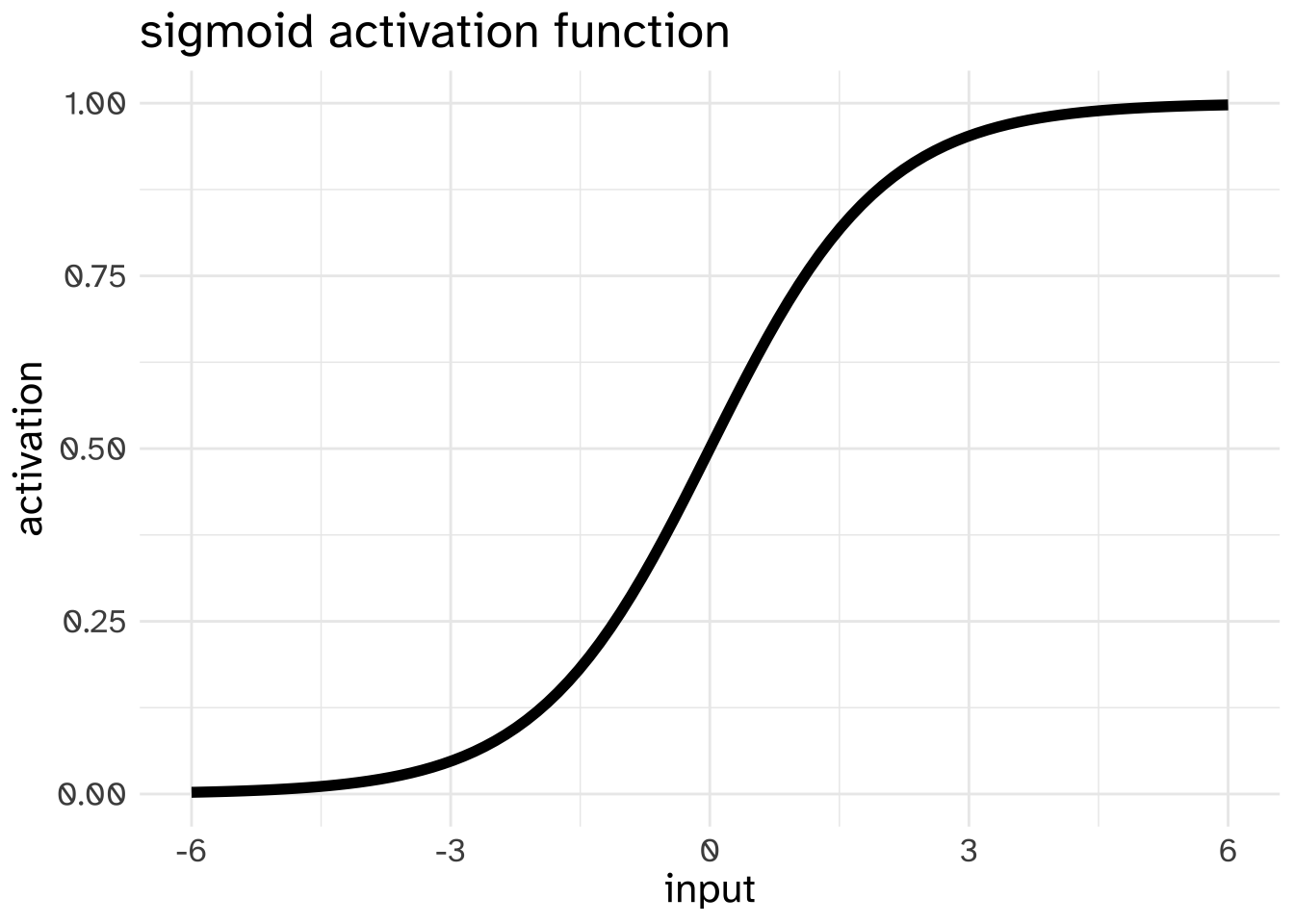
If the outcome of taking the dot product of input data and weights and adding the bias was 0, a node using the sigmoid activation function would pass 0.5 onto the next layer. It was 6, the node would pass on a value close to 1 to the next layer.
Another commonly used activation function is the “Rectified Linear Unit” or ReLU. This pass on whatever value comes in if it is greater than 0, and pass on 0 otherwise.
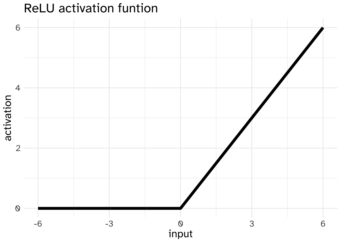
One reason why the ReLU has been preferred over the sigmoid for some purposes is that it can be more useful for gradient descent, for reasons that involve talking about more calculus than we can get into here.
Deciding on the model
Let’s build a model that has two hidden layers, each with 10 nodes that use the ReLU activation function
import tensorflow as tfHere’s how that looks in Tensorflow
model = tf.keras.models.Sequential([
  tf.keras.layers.Dense(10, input_shape=(4,), activation = "relu"),
  tf.keras.layers.Dense(10, activation='relu'),
  tf.keras.layers.Dense(5)
])
The model is initialized with random weights, and we can preview the kind of outputs we get
raw_output = model(X_train[0:3])
raw_output
<tf.Tensor: shape=(3, 5), dtype=float32, numpy=
array([[ 0.04585112, -0.13618417, -0.20613343, -0.02187469, -0.0069646 ],
[-0.00922366, 0.07055292, 0.01235281, -0.06401903, -0.0344503 ],
[-0.02687357, 0.1050203 , 0.1833 , 0.02528077, -0.05633993]],
dtype=float32)>Each row is the number that winds up in the the output node. We can convert them to probabilities with softmax:
tf.nn.softmax(raw_output)<tf.Tensor: shape=(3, 5), dtype=float32, numpy=
array([[0.22252385, 0.18548964, 0.17295818, 0.20795226, 0.21107607],
[0.1989407 , 0.21546173, 0.20327976, 0.18833293, 0.19398485],
[0.18520641, 0.21131817, 0.22852476, 0.19512206, 0.17982867]],
dtype=float32)>We can also get the predicted category label with argmax/
pred = tf.math.argmax(raw_output, axis = 1)
pred.numpy()
array([0, 1, 2])These predicted category labels aren’t good predictions for the actual category labels.
y_train[0:3]array([1, 4, 3])Loss Function
Next, we need to decide on the loss function, or how we’re going to measure how badly our predictions match the data. Since we’re giving the model integer labels and getting back a list of un-scaled weights for each possible category, the appropriate loss function here is Sparse Categorical Cross Entropy
loss_fn = tf.keras.losses.SparseCategoricalCrossentropy(from_logits=True)loss_fn(y_true=y_train[0:3], y_pred=raw_output)<tf.Tensor: shape=(), dtype=float32, numpy=1.6529537>There are a lot of loss functions available in TensorFlow, and they’re all just kind of listed here: https://www.tensorflow.org/api_docs/python/tf/keras/losses
Here’s some rules of thumb for deciding on a specific loss function
| You’re predicting… | which is coded as… | so use… |
|---|---|---|
| Multiple categories | integers (e.g. [0, 3, 1, 2, 2] |
Sparse Categorical Cross Entropy |
| Multiple categories | one hot encoding (e.g. |
Categorical Cross Entropy |
| A binary outcome | A 0 or a 1 |
Binary Cross Entropy |
| A continuous value | A numeric value | Mean Squared Error |
Optimizer
Next, we need to decide on the “optimizer” we’re going to use. On every iteration, the model is going to estimate the gradient of the loss for every model parameter. The optimizer controls how that gradient is used. A popular one is the Adam optimizer.
optim_fn = tf.keras.optimizers.Adam()Training the Model!
First, we need to “compile” the model, telling it which optimizer and loss function we want to use, as well as any additional metrics we want it to keep track of as it trains.
model.compile(optimizer=optim_fn,
              loss=loss_fn,
              metrics=['accuracy'])
Then, we fit the model, telling it to use the training data, and how many epochs to train for. I’m also telling the model to automatically select out 20% of the training data to use as a “validation” dataset. The model will see how well it does on the validation data after every epoch, but won’t use it to actually train on.
All of the updated weights are kept inside the model object. I’m assigning the ouput to history, which will now contain a dictionary of how of the losses and metrics changed after each epoch.
history = model.fit(X_train, y_train,
                    epochs=500, verbose = 0,
                    validation_split = 0.2)
Visualizing and evaluating the model
So, how’d we do? We can look at some plots to see.
training_history = pd.DataFrame.from_dict(history.history)nrow = training_history.shape[0]
training_history["epoch"] = list(range(nrow))loss_plot = px.line(training_history, x = "epoch", y = ["loss", "val_loss"], title = "loss over epochs")
loss_plot.show()acc_plot = px.line(training_history, x = "epoch", y = ["accuracy", "val_accuracy"], title ="accuracy over epochs")
acc_plot.show()To really evaluate how well we’ve done, we’ll need to compare these accuracy measures to some baseline, wrong models. Here’s some options:
- Random choice out of 5 labels.
- Choose the most frequent label
- Randomly scramble the labels.
The random choice out of 5 labels would be 1/5 = 0.2.
random_choice = 1/5
random_choice0.2# getting probabilty of most frequent
from collections import Counter
Counter(y_train)Counter({3: 786, 1: 408, 0: 402, 4: 158, 2: 146})most_common_prob = Counter(y_train).most_common()[0][1]/len(y_train)
most_common_prob0.41368421052631577# getting the accuracy of just shuffling the labels
shuff_array = np.copy(y_train)
n_shuffle = 1000
shuff_total = 0
for x in range(n_shuffle):
np.random.shuffle(shuff_array)
shuff_total += (shuff_array == y_train).mean()
shuff_mean = shuff_total/n_shuffle
shuff_mean0.2747221052631582acc_plot_comp = (px.line(training_history,
x = "epoch",
y = ["accuracy", "val_accuracy"],
title ="accuracy over epochs")
.update_yaxes(range=[0, 1])
.add_hline(y = random_choice,
line_color = "steelblue",
annotation_text="random choice",
annotation_position = "top left")
.add_hline(y = most_common_prob,
line_color = "firebrick",
annotation_text="most common label",
annotation_position = "top left")
.add_hline(y = shuff_mean,
line_color = "green",
annotation_text="label shuffle",
annotation_position = "top left")
)
acc_plot_comp.show()test_pred = model(X_test)
test_pred_int = tf.math.argmax(test_pred, axis = 1).numpy()
(test_pred_int == y_test).mean()0.6239495798319328More Layers?
Would adding more layers improve the accuracy?
model2 = tf.keras.models.Sequential([
  tf.keras.layers.Dense(10, input_shape=(4,), activation = "relu"),
  tf.keras.layers.Dense(10, activation='relu'),
  tf.keras.layers.Dense(10, activation='relu'),
  tf.keras.layers.Dense(5)
])model2.compile(optimizer=optim_fn,
loss=loss_fn,
metrics=['accuracy'])history2 = model2.fit(X_train, y_train,
epochs=500, verbose = 0,
validation_split = 0.2)training_history2 = pd.DataFrame.from_dict(history2.history)
training_history2["epoch"] = range(500)acc_plot_comp2 = (px.line(training_history2,
x = "epoch",
y = ["accuracy", "val_accuracy"],
title ="accuracy over epochs")
.update_yaxes(range=[0, 1])
.add_hline(y = random_choice,
line_color = "steelblue",
annotation_text="random choice",
annotation_position = "top left")
.add_hline(y = most_common_prob,
line_color = "firebrick",
annotation_text="most common label",
annotation_position = "top left")
.add_hline(y = shuff_mean,
line_color = "green",
annotation_text="label shuffle",
annotation_position = "top left")
)
acc_plot_comp2.show()Dropout?
model3 = tf.keras.models.Sequential([
  tf.keras.layers.Dense(100, input_shape=(4,), activation = "relu"),
  tf.keras.layers.Dropout(0.5),
  tf.keras.layers.Dense(100, activation='relu'),
  tf.keras.layers.Dropout(0.5),
  tf.keras.layers.Dense(100, activation='relu'),
  tf.keras.layers.Dropout(0.5),
  tf.keras.layers.Dense(100, activation='relu'),
  tf.keras.layers.Dropout(0.5),
  tf.keras.layers.Dense(5)
])model3.compile(optimizer=optim_fn,
loss=loss_fn,
metrics=['accuracy'])history3 = model3.fit(X_train, y_train,
epochs=500, verbose = 0,
validation_split = 0.2)training_history3 = pd.DataFrame.from_dict(history3.history)
training_history3["epoch"] = range(500)
acc_plot_comp3 = (px.line(training_history3,
x = "epoch",
y = ["accuracy", "val_accuracy"],
title ="accuracy over epochs")
.update_yaxes(range=[0, 1])
.add_hline(y = random_choice,
line_color = "steelblue",
annotation_text="random choice",
annotation_position = "top left")
.add_hline(y = most_common_prob,
line_color = "firebrick",
annotation_text="most common label",
annotation_position = "top left")
.add_hline(y = shuff_mean,
line_color = "green",
annotation_text="label shuffle",
annotation_position = "top left")
)
acc_plot_comp3.show()