Normalization Overview • tidynorm

Introduction to the problem

library(tidynorm)
library(dplyr)
library(tidyr)

library(ggplot2)
library(ggdensity)

color palette

options(
  ggplot2.discrete.colour = c(
    lapply(
      1:6, 
      \(x) c("#4477AA", "#EE6677", "#228833", 
             "#CCBB44", "#66CCEE", "#AA3377")[1:x]
    )
  ),
  ggplot2.discrete.fill = c(
    lapply(
      1:6, 
      \(x) c("#4477AA", "#EE6677", "#228833", 
             "#CCBB44", "#66CCEE", "#AA3377")[1:x]
    )
  )  
)

theme_set(
  theme_minimal(base_size = 16)+
    theme(
      panel.grid = element_blank()
    )
)

Vowel formant frequencies are heavily influenced by speakers’ vocal tract length, such that equivalent vowels can have dramatically different formant frequencies

speaker_data |> 
  summarise(
    .by = c(speaker, vowel),
    across(
      F1:F3,
      \(x)mean(x, na.rm = T)
    )
  ) ->
  speaker_means

Plotting Code

speaker_means |> 
  filter(
    vowel %in% c("IY","UW","AE","AA")
  ) |> 
  ggplot(
    aes(F2, F1)
  )+
  geom_label(
    aes(
      label = vowel,
      fill = speaker
    ),
    color = "white"
  )+
  scale_y_reverse()+
  scale_x_reverse()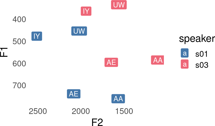

Vowel Comparison

speaker_means |> 
  filter(
    vowel %in% c("IY","UW","AE","AA")
  ) |>   
  pivot_longer(
    F1:F3,
    names_to = ".formant_name",
    values_to = ".formant"
  ) |> 
  pivot_wider(
    names_from = vowel,
    values_from = .formant
  ) |> 
  arrange(
    .formant_name
  )

# A tibble: 6 × 6
  speaker .formant_name    IY    AA    AE    UW
  <chr>   <chr>         <dbl> <dbl> <dbl> <dbl>
1 s01     F1             477.  761.  739.  454.
2 s03     F1             364.  585.  596.  335.
3 s01     F2            2513. 1568. 2084. 2021.
4 s03     F2            1941. 1109. 1648. 1560.
5 s01     F3            3264. 2938. 3095. 3081.
6 s03     F3            2726. 2269. 2518. 2412.

When conducting an analysis that combines multiple different speakers’ data together, we often want to factor out this vocal tract length difference, so that we can instead focus our attention on the relative values of these vowel frequencies within speakers.

An example

When speakers s01 and s03 in the speakers_data data set have very different vowel spaces that differ both in the location of their center points, and scaling.

Plotting code

speaker_centers <- speaker_data |> 
  summarise(
    .by = speaker,
    across(
      F1:F3,
      ~mean(.x, na.rm = T)
    )
  )

speaker_data |> 
  ggplot(
    aes(F2, F1, color = speaker)
  )+
  stat_hdr(
    probs = c(0.95, 0.8, 0.5),
    fill = NA,
    alpha = 1,
    linewidth = 1
  )+
  geom_point(
    data = speaker_centers,
    size = 5
  )+
  scale_x_reverse()+
  scale_y_reverse()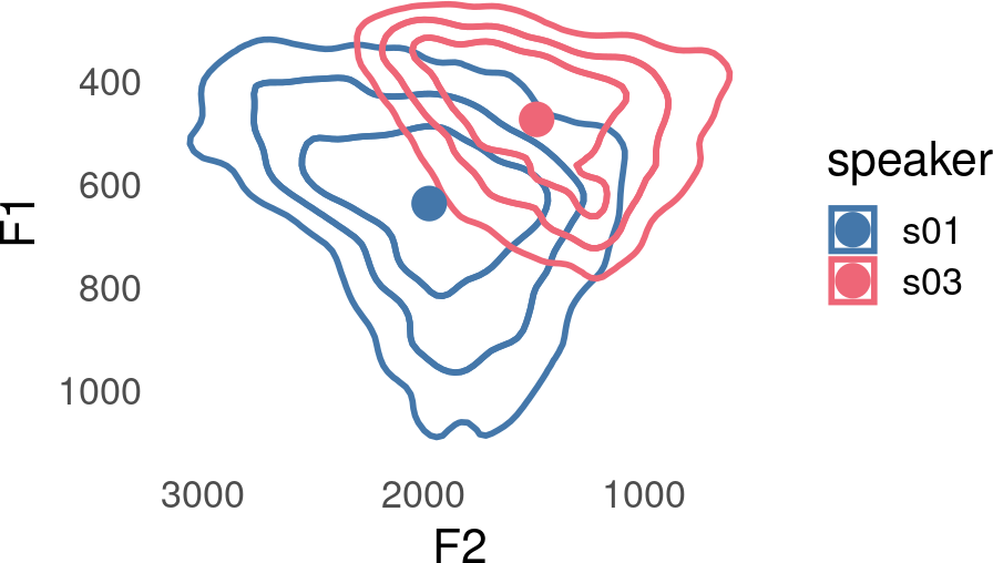

One approach to moving speakers center points to a common location is to subtract the mean from both F1 and F2.

speaker_data_centered <- speaker_data |> 
 mutate(
    .by = speaker,
    across(
      F1:F3,
      ~.x - mean(.x, na.rm = T)
    )
  )

Now s01 and s03’s center points have a common location, but the scale of s03’s vowels is still smaller than s01’s.

Plotting code

speaker_data_centered |> 
  ggplot(
    aes(F2, F1, color = speaker)
  ) +
  stat_hdr(
    probs = c(0.95, 0.8, 0.5),
    fill = NA,
    alpha = 1,
    linewidth = 1
  )+
  geom_point(
    data = tibble(),
    aes(x = 0, y = 0),
    color = "black",
    size = 5,
  )+
  scale_y_reverse()+
  scale_x_reverse()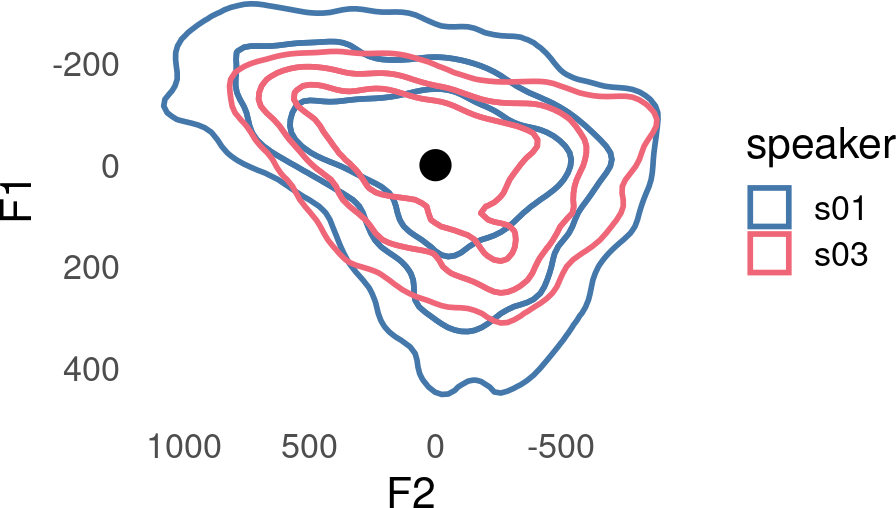

An approach to putting speakers’ vowel spaces on a common scale is to divide by the standard deviation.

speaker_data_scaled <- speaker_data |> 
  mutate(
    .by = speaker,
    across(
      F1:F3,
      ~.x/sd(.x, na.rm = T)
    )
  )

The result is two vowel spaces with center points in the same location, and on a common scale.

Plotting code

speaker_data_scaled |> 
  mutate(
    .by = speaker,
    across(
      F1:F3,
      ~(.x - mean(.x, na.rm = T))/sd(.x, na.rm = T)
    )
  ) |> 
  ggplot(
    aes(F2, F1, color = speaker)
  )+
 stat_hdr(
    probs = c(0.95, 0.8, 0.5),
    fill = NA,
    alpha = 1,
    linewidth = 1
  )+
  geom_point(
    data = tibble(),
    aes(x = 0, y = 0),
    color = "black",
    size = 5,
  )+  
  scale_y_reverse()+
  scale_x_reverse()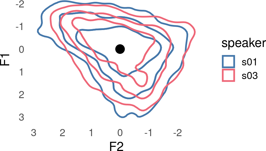

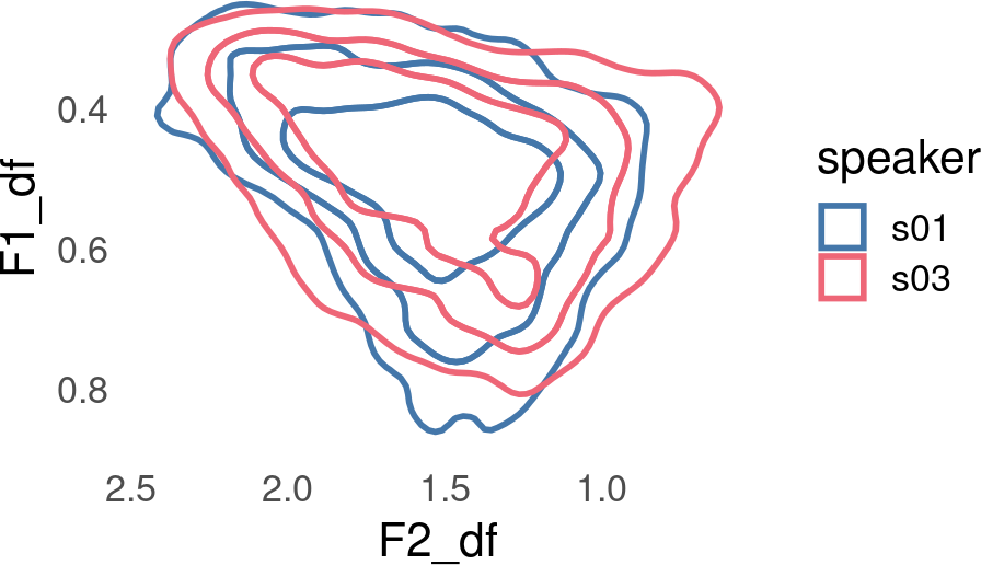
Generalizing Normalization Procedures

All speaker normalization techniques involves some form of Location shift (L), Scaling (S), or both. If F is an unnormalized formant value, and \hat{F} is the normalized value, then:

\hat{F} = \frac{F-L}{S}

The primary differences between normalization methods are:

The use of across-the-board data transformations.
The calculation function for L and S.
The scope of calculating L and S.

The example above is also known as Lobanov Normalization (see norm_lobanov()). The norm_generic() function allows for flexible definitions of normalization procedures with this in mind.

Examples

\DeltaF

The \DeltaF method was described in Johnson (2020).

It uses no across-the-board data transformation.
It uses a scaling factor S called \DeltaF, which is the mean across all formants of the formant frequency in Hz, divided by the formant number minus 0.5.
S is calculated across all formants

S = \Delta F = \text{mean}\left(\frac{F_{ij}}{i-0.5}\right)

This can be expressed with norm_generic() like so

speaker_data |> 
  norm_generic(
    F1:F3,
    .by = speaker,
    .by_formant = FALSE,
    .by_token = FALSE,
    .L = 0,
    .S = mean(
      .formant/(.formant_num - 0.5), 
      na.rm = T
    ),
    .names = "{.formant}_df"
  )->
  speaker_df_norm

Normalization info
• normalized `F1`, `F2`, and `F3`
• normalized values in `F1_df`, `F2_df`, and `F3_df`
• grouped by `speaker`
• formant extrinsic

ggplot(
  speaker_df_norm, 
  aes(F2_df, F1_df, color = speaker)
)+
  stat_hdr(
    probs = c(0.95, 0.8, 0.5),
    fill = NA,
    alpha = 1,
    linewidth = 1
  )+
  scale_y_reverse()+
  scale_x_reverse()

Johnson, Keith. 2020. “The ΔF Method of Vocal Tract Length Normalization for Vowels.” Laboratory Phonology: Journal of the Association for Laboratory Phonology 11 (11): 10. https://doi.org/10.5334/labphon.196.