Because densityarea can return sf polygons, this can allow you to use its functionality (see this cheat sheet for some examples).
Density polygons as simple features
As a first example, we’ll estimate how much different data clusters
overlap in the s01 dataset.
We’ll focus on the vowels iy, ey,
o and oh which correspond to the following
lexical classes:
| vowel label | lexical class |
|---|---|
iy |
Fleece |
ey |
Face |
o |
Lot |
oh |
Thought |
Within this subset of vowel categories, we’ll get the 80% probability
density estimate as sf::st_polygon()s.
vowel_subset |>
  group_by(plt_vclass) |>
  reframe(
    density_polygons(lF2,
                     lF1,
                     probs = 0.8,
                     as_sf = TRUE)
  ) |>
  st_sf()->
  vowel_polygons

vowel_polygons
#> Simple feature collection with 4 features and 3 fields
#> Geometry type: POLYGON
#> Dimension:     XY
#> Bounding box:  xmin: -8.050893 ymin: -7.037138 xmax: -6.996794 ymax: -5.820745
#> CRS:           NA
#> # A tibble: 4 × 4
#>   plt_vclass level_id  prob                                             geometry
#>   <chr>         <int> <dbl>                                            <POLYGON>
#> 1 ey                1   0.8 ((-7.840111 -6.222708, -7.842276 -6.221536, -7.8515…
#> 2 iy                1   0.8 ((-7.862895 -5.820745, -7.872822 -5.820892, -7.8799…
#> 3 o                 1   0.8 ((-7.351372 -6.23354, -7.365699 -6.233222, -7.38002…
#> 4 oh                1   0.8 ((-7.231025 -6.420727, -7.240256 -6.419138, -7.2494…
We can plot these directly by using the sf::geom_sf()
geom for ggplot2.
ggplot(vowel_polygons) +
  geom_sf(
    aes(fill = plt_vclass),
    alpha = 0.6
  ) +
    scale_fill_brewer(palette = "Dark2")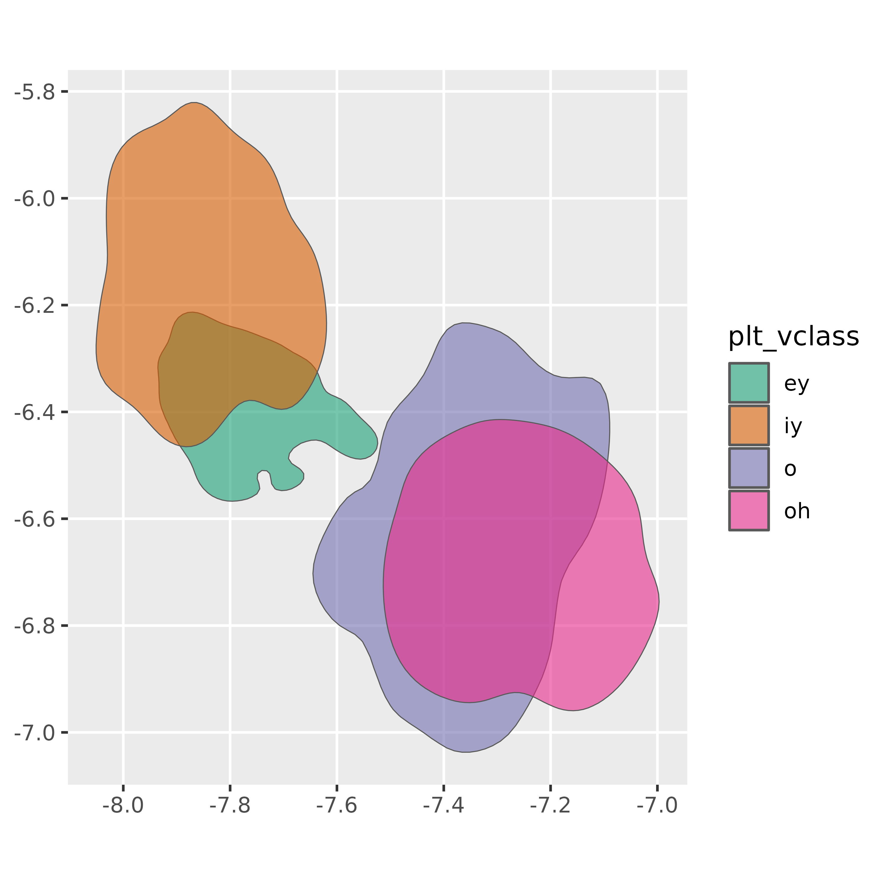
Initial {sf} operations
All of the sf operations for geometries are available
to use on vowel_polygons. For example, we can get the area
of each polygon, with sf::st_area() and use it in
plotting.
ggplot(vowel_polygons) +
  geom_sf(
    aes(fill = area),
    alpha = 0.6
  )+
  scale_fill_viridis_c()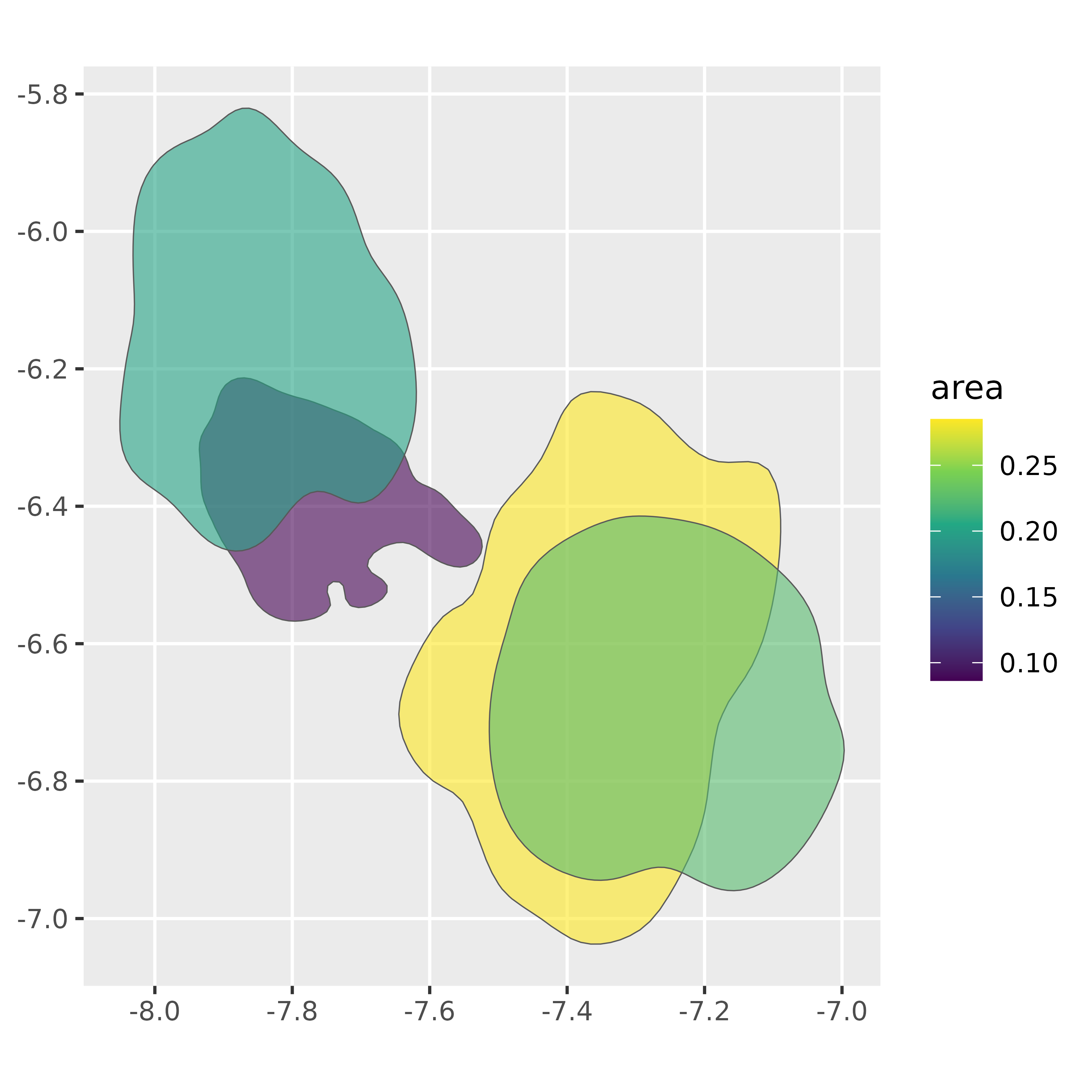
Or, we can get the polygon centroids and plot them.
vowel_polygons |>
  st_centroid() |>
  ggplot()+
    geom_sf_label(
      aes(label = plt_vclass,
          color = plt_vclass,
          size = area)
    )+
    scale_color_brewer(palette = "Dark2")+
    coord_fixed()
#> Warning: st_centroid assumes attributes are constant over geometries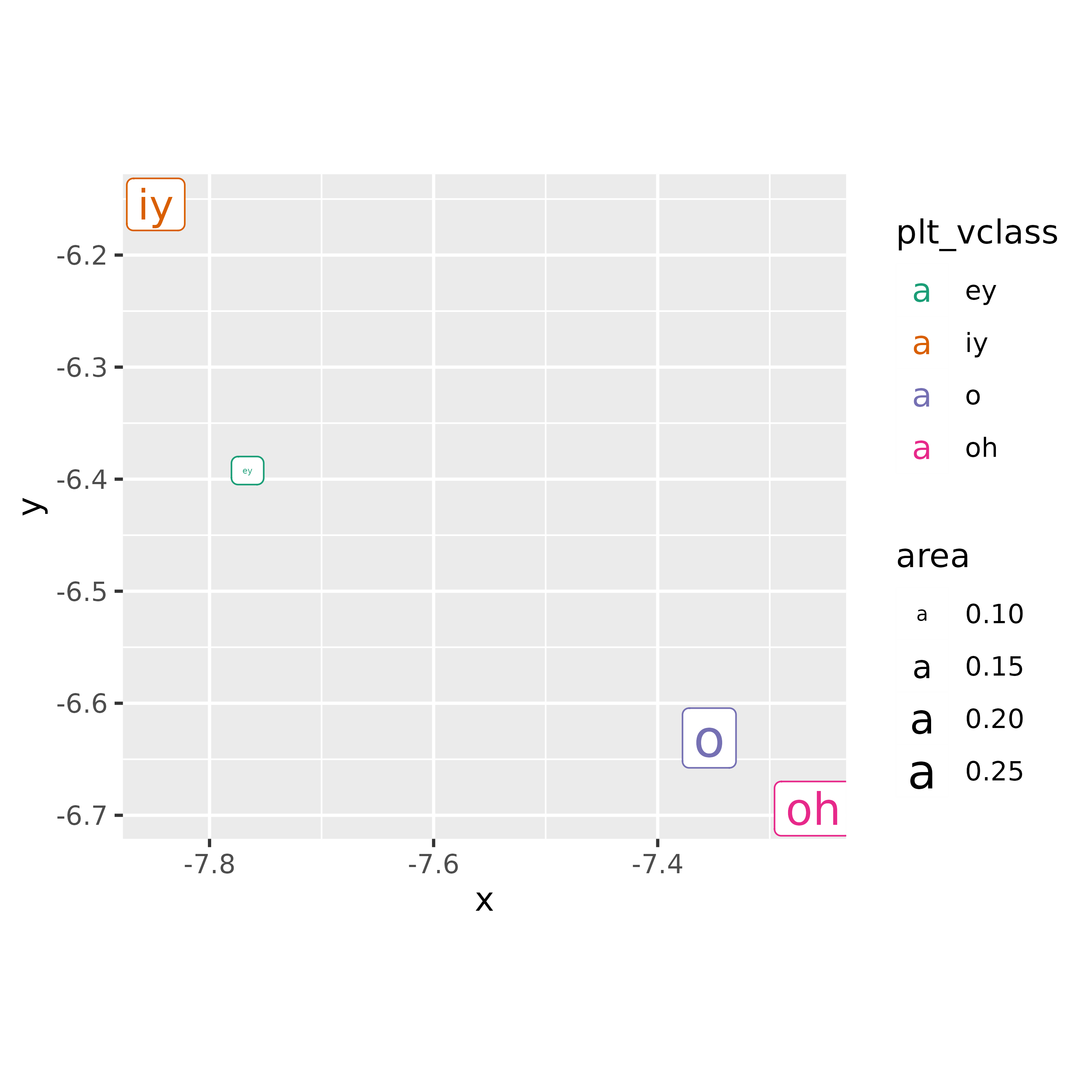
Getting overlaps
To use the density polygons like “cookie cutters” on each other, we
need to use st_intersections().
vowel_polygons |>
  st_intersection() ->
  vowel_intersections

vowel_intersections
#> Simple feature collection with 6 features and 6 fields
#> Geometry type: POLYGON
#> Dimension:     XY
#> Bounding box:  xmin: -8.050893 ymin: -7.037138 xmax: -6.996794 ymax: -5.820745
#> CRS:           NA
#> # A tibble: 6 × 7
#>   plt_vclass level_id  prob   area n.overlaps origins                   geometry
#>   <chr>         <int> <dbl>  <dbl>      <int> <list>                   <POLYGON>
#> 1 ey                1   0.8 0.0865          1 <int>   ((-7.63623 -6.326645, -7.…
#> 2 ey                1   0.8 0.0865          2 <int>   ((-7.896883 -6.458929, -7…
#> 3 iy                1   0.8 0.202           1 <int>   ((-7.902604 -6.461049, -7…
#> 4 o                 1   0.8 0.285           1 <int>   ((-7.236759 -6.940033, -7…
#> 5 o                 1   0.8 0.285           2 <int>   ((-7.093493 -6.493589, -7…
#> 6 oh                1   0.8 0.224           1 <int>   ((-7.092569 -6.49308, -7.…
This data frame contains a polygon for each unique intersection of
the input polygons, with a new n.overlaps column.
ggplot(vowel_intersections) +
  geom_sf(
    aes(fill = n.overlaps)
  )+
  scale_fill_viridis_c()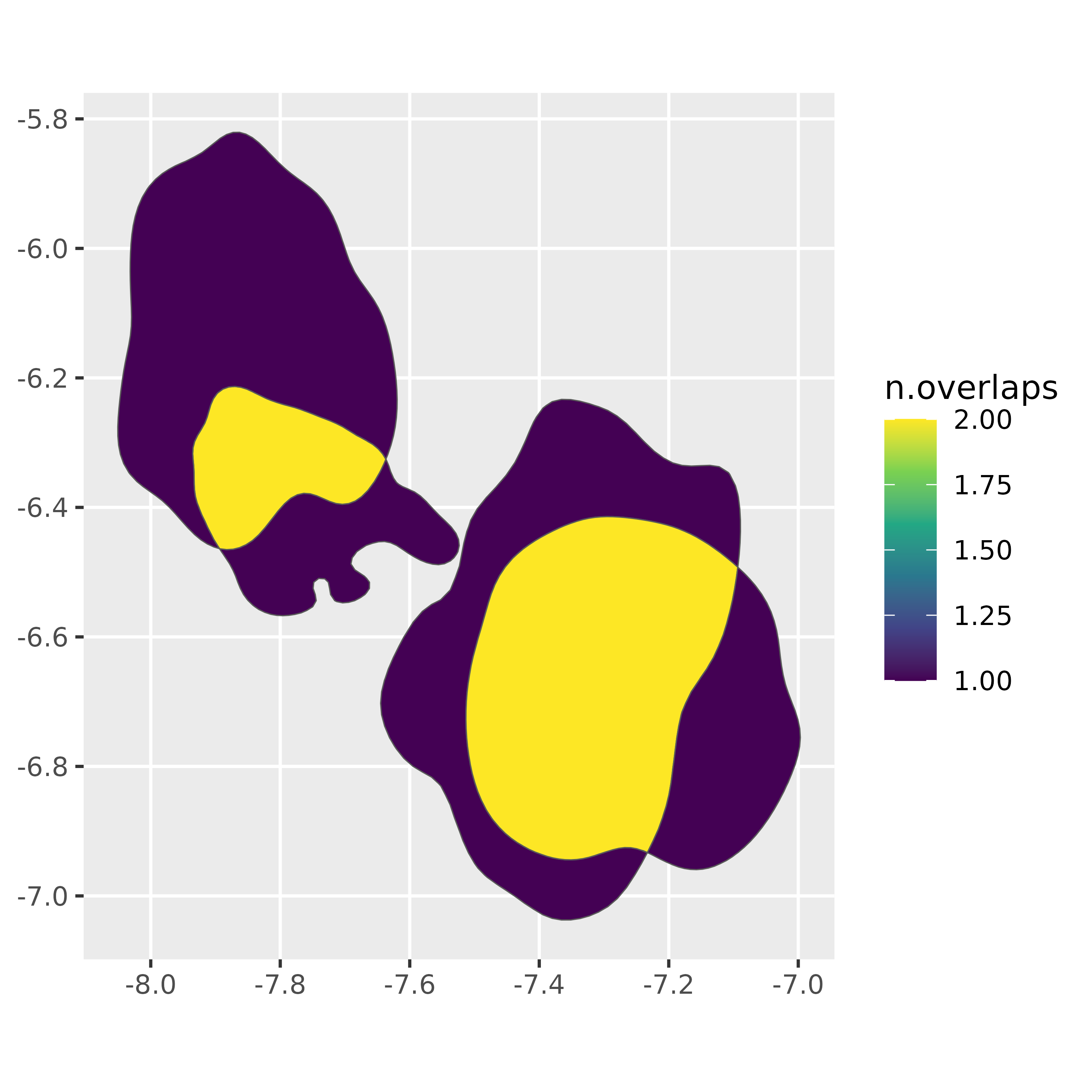
The labels of the new overlapping regions aren’t very informative,
but we can create some new labels by using the indices in the
origins column.
new_label <- function(indices, labels){
  str_c(labels[indices],
        collapse = "~")
}
vowel_intersections |>
  mutate(
    groups = map_chr(
      origins,
      .f = new_label,
      labels = vowel_polygons$plt_vclass
    )
  ) |>
  relocate(groups, .after = plt_vclass)->
  vowel_intersections

vowel_intersections
#> Simple feature collection with 6 features and 7 fields
#> Geometry type: POLYGON
#> Dimension:     XY
#> Bounding box:  xmin: -8.050893 ymin: -7.037138 xmax: -6.996794 ymax: -5.820745
#> CRS:           NA
#> # A tibble: 6 × 8
#>   plt_vclass groups level_id  prob   area n.overlaps origins
#>   <chr>      <chr>     <int> <dbl>  <dbl>      <int> <list>
#> 1 ey         ey            1   0.8 0.0865          1 <int [1]>
#> 2 ey         ey~iy         1   0.8 0.0865          2 <int [2]>
#> 3 iy         iy            1   0.8 0.202           1 <int [1]>
#> 4 o          o             1   0.8 0.285           1 <int [1]>
#> 5 o          o~oh          1   0.8 0.285           2 <int [2]>
#> 6 oh         oh            1   0.8 0.224           1 <int [1]>
#> # ℹ 1 more variable: geometry <POLYGON>
ggplot(vowel_intersections)+
  geom_sf(
    aes(fill = groups)
  )+
  scale_fill_brewer(palette = "Dark2")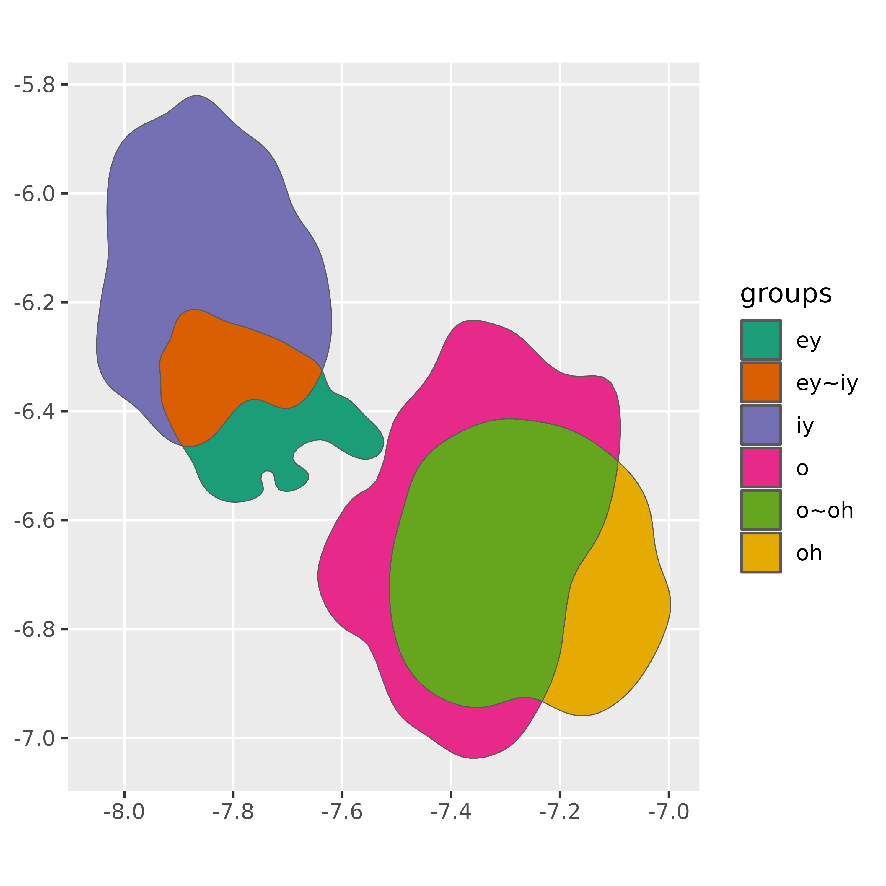
We can also calculate the areas of these new polygons, and compare
them to the original areas (which have been preserved in
areas.
vowel_intersections |>
  mutate(
    group_area = st_area(geometry),
    overlapped_proportion = 1-(group_area/area)
  ) |>
  filter(n.overlaps == 1) |>
  ggplot(
    aes(plt_vclass, overlapped_proportion)
  )+
    geom_col()+
    ylim(0,1)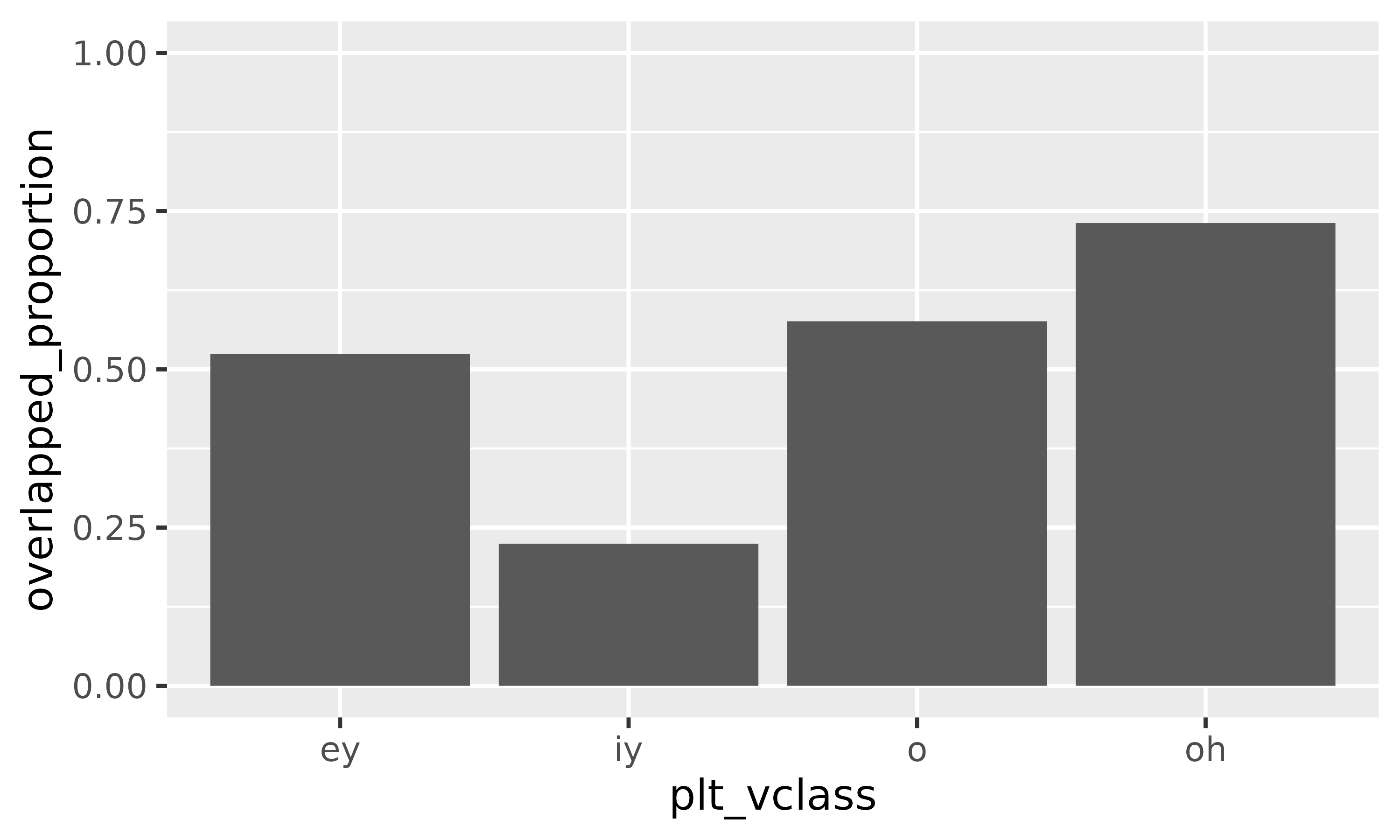
Spatial filters
There are also a number of spatial filters and merges that can be used interestingly if the original data points are also converted to sf objects.
s01 |>
  sfheaders::sf_point(
    x = "lF2",
    y = "lF1",
    keep = TRUE
  ) ->
  s01_sf

s01_sf
#> Simple feature collection with 4245 features and 10 fields
#> Geometry type: POINT
#> Dimension:     XY
#> Bounding box:  xmin: -8.095446 ymin: -7.335764 xmax: -6.541463 ymax: -5.439817
#> CRS:           NA
#> First 10 features:
#>    name age sex     word vowel plt_vclass ipa_vclass    F1     F2  dur
#> 1   s01   y   f     OKAY    EY        eyF        ejF 763.5 2088.1 0.20
#> 2   s01   y   f       UM    AH         uh          ʌ 699.5 1881.3 0.19
#> 3   s01   y   f      I'M    AY         ay         aj 888.8 1934.1 0.07
#> 4   s01   y   f    LIVED    IH          i          ɪ 555.5 1530.5 0.05
#> 5   s01   y   f       IN    IH          i          ɪ 612.2 2323.4 0.06
#> 6   s01   y   f COLUMBUS    AH          @          ə 612.4 1903.7 0.07
#> 7   s01   y   f       MY    AY         ay         aj 578.4 1959.3 0.09
#> 8   s01   y   f   ENTIRE    IH          i          ɪ 529.9 2332.1 0.08
#> 9   s01   y   f   ENTIRE    ER        *hr         ə˞ 538.4 1682.8 0.18
#> 10  s01   y   f     LIFE    AY        ay0        aj0 744.6 1702.1 0.15
#>                       geometry
#> 1   POINT (-7.64401 -6.637913)
#> 2  POINT (-7.539718 -6.550366)
#> 3  POINT (-7.567397 -6.789872)
#> 4   POINT (-7.33335 -6.319869)
#> 5  POINT (-7.750787 -6.417059)
#> 6  POINT (-7.551555 -6.417386)
#> 7  POINT (-7.580343 -6.360266)
#> 8  POINT (-7.754524 -6.272688)
#> 9  POINT (-7.428214 -6.288602)
#> 10 POINT (-7.439618 -6.612847)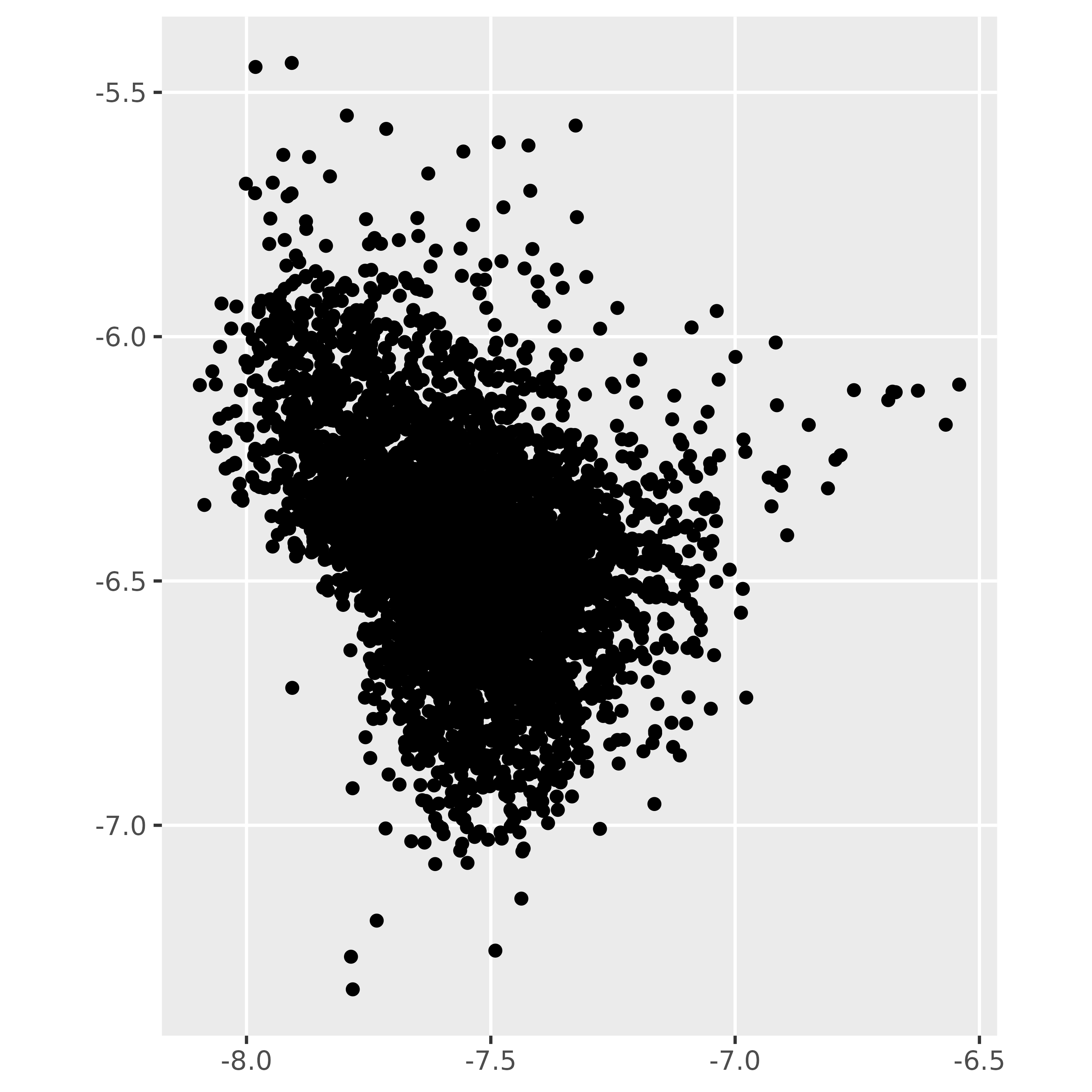
Next, we can get the density polygon for a single vowel,.
s01 |>
  filter(plt_vclass == "iy") |>
  reframe(
    density_polygons(lF2, lF1, probs = 0.8, as_sf =T)
  ) |>
  st_sf()->
  iy_sf
Spatial filter
Let’s get all of the points in s01_sf that are “covered
by” the iy_sf polygon.
s01_sf |>
  st_filter(
    iy_sf,
    .predicate = st_covered_by
  )->
  covered_by_iy
covered_by_iy |>
  mutate(plt_vclass = plt_vclass |>
           fct_infreq() |>
           fct_lump_n(5)) |>
  ggplot()+
    geom_sf(data = iy_sf)+
    geom_sf(aes(color = plt_vclass))+
    scale_color_brewer(palette = "Dark2")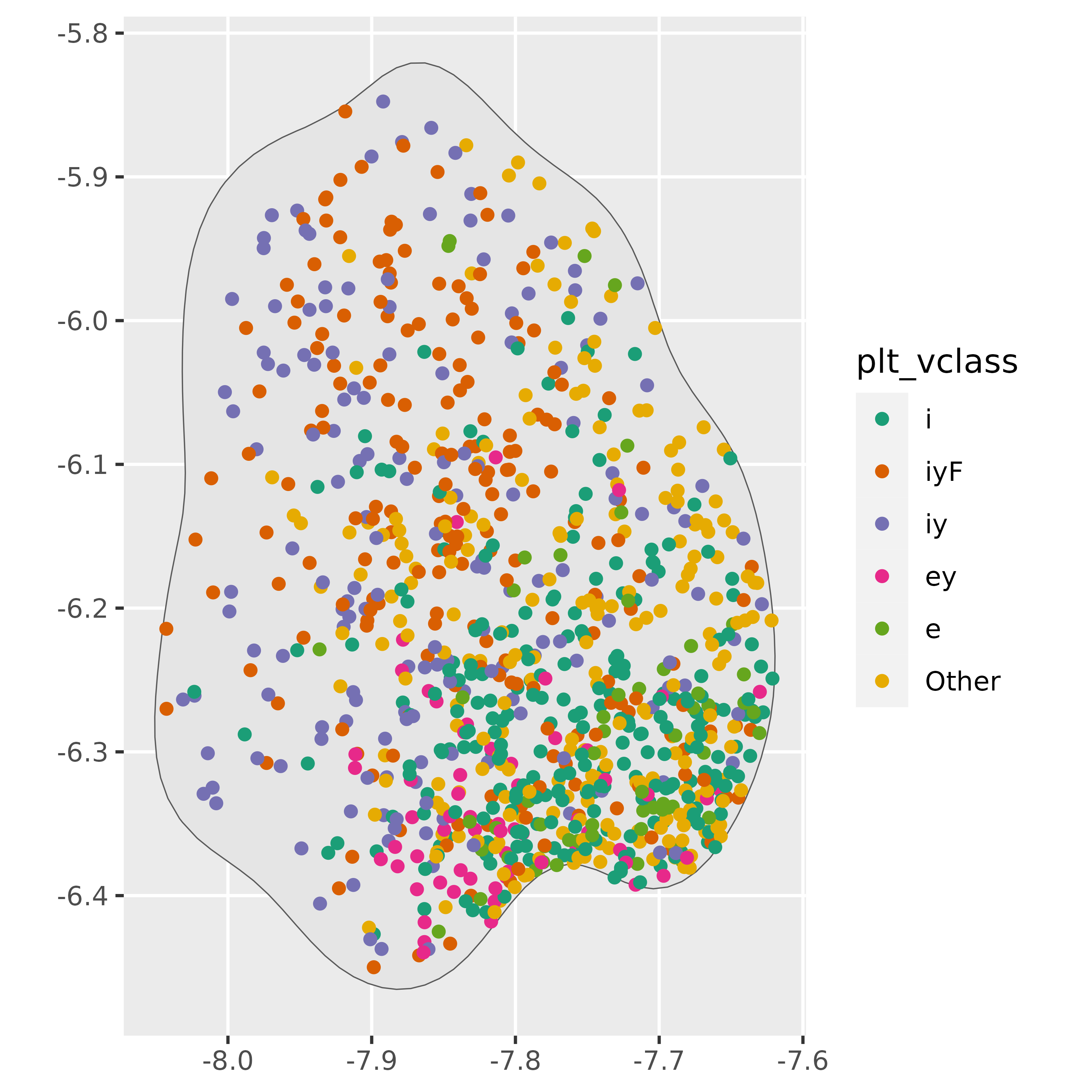
Obviously, the 80% probability density area for iy is
not a homogeneous region.
covered_by_iy |>
  mutate(plt_vclass = plt_vclass |>
           fct_infreq() |>
           fct_lump_n(5)) |>
  count(plt_vclass) |>
  ggplot(aes(plt_vclass, n))+
    geom_col(
      aes(fill = plt_vclass)
    )+
    scale_fill_brewer(palette = "Dark2")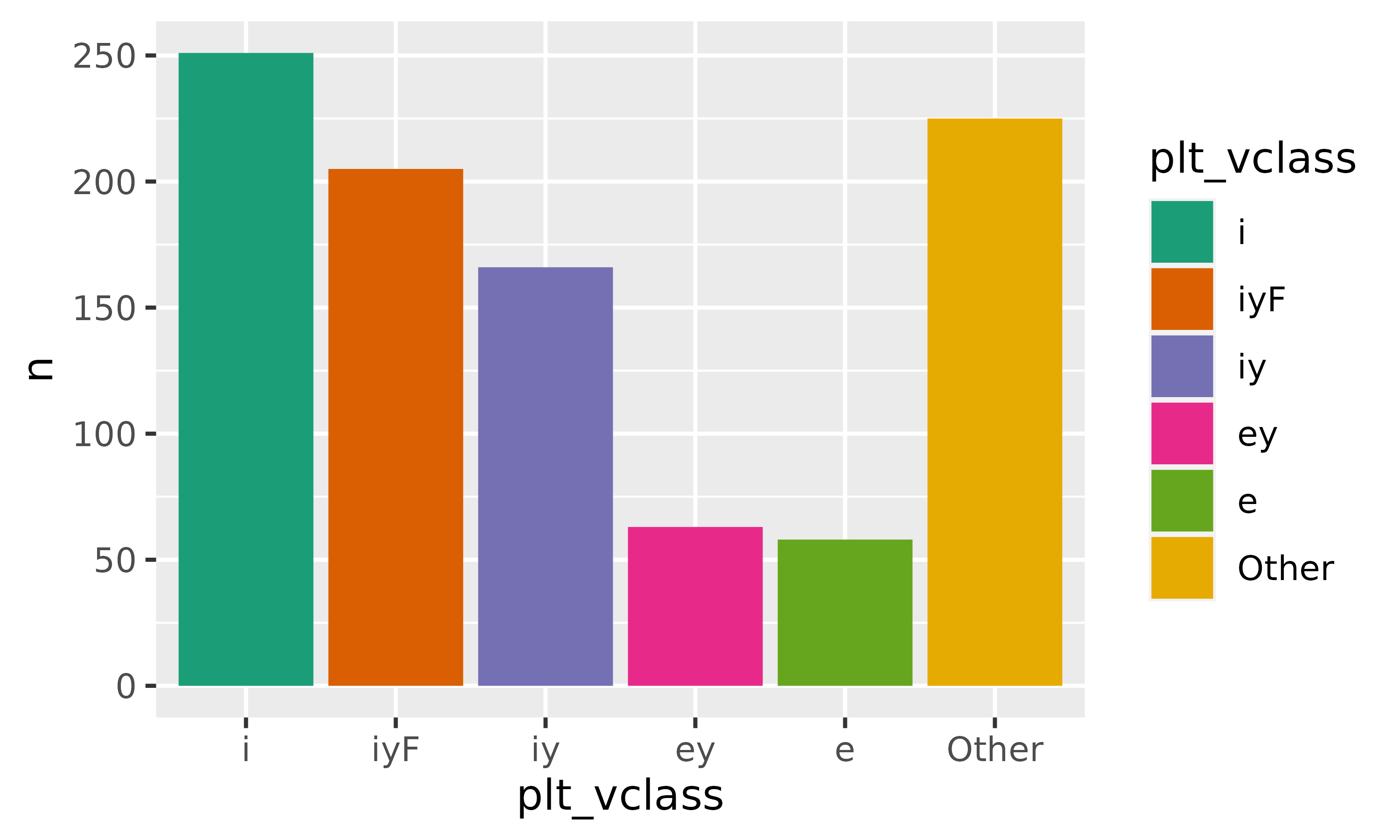
Spatial join
Let’s see which vowel category a random vowel token is close to.
set.seed(100)
s01_sf |>
  slice_sample(n = 1)->
  rand_vowel

rand_vowel
#> Simple feature collection with 1 feature and 10 fields
#> Geometry type: POINT
#> Dimension:     XY
#> Bounding box:  xmin: -7.440205 ymin: -6.508322 xmax: -7.440205 ymax: -6.508322
#> CRS:           NA
#>   name age sex word vowel plt_vclass ipa_vclass    F1     F2  dur
#> 1  s01   y   f LIKE    AY        ay0        aj0 670.7 1703.1 0.09
#>                      geometry
#> 1 POINT (-7.440205 -6.508322)
Then, we’ll get density polygons at a few different probability points for all vowels.
s01 |>
  group_by(plt_vclass) |>
  reframe(
    density_polygons(
      lF2,
      lF1,
      probs = ppoints(5),
      range_mult = 0.5,
      as_sf = T
    )
  ) |>
  st_sf() ->
  vowel_probs
There are 5 probability level polygons for each vowel category in
vowel_probs. We join the random vowel’s data onto this set
of polygons with st_join().
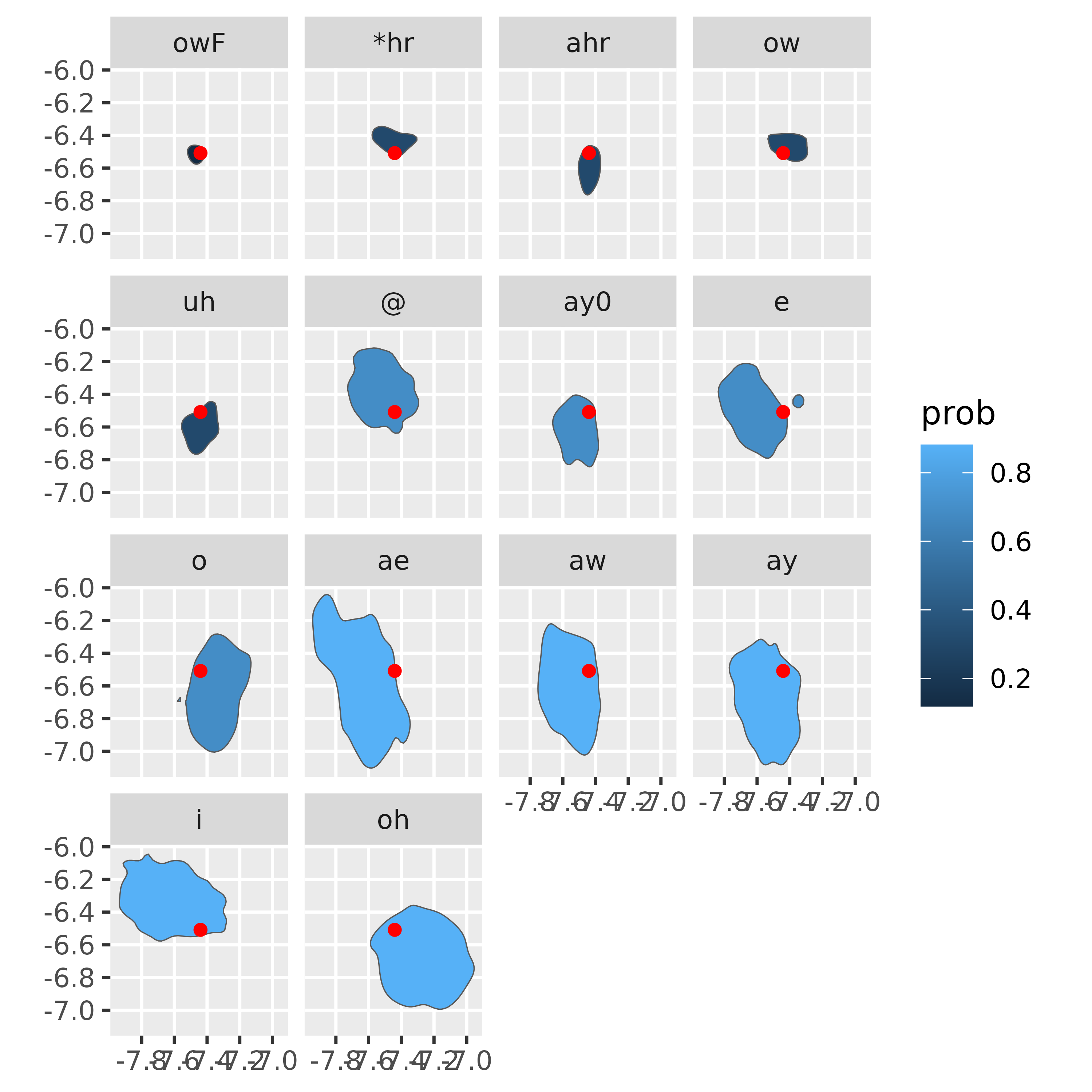
Now, for each vowel category in this new data frame, let’s get the smallest probability polygon (i.e. where the random point is closest to the center probability mass).
vowel_within |>
  group_by(plt_vclass.x) |>
  filter(prob == min(prob)) |>
  ungroup() |>
  mutate(plt_vclass = fct_reorder(plt_vclass.x, prob)) ->
  vowel_min_prob
vowel_min_prob |>
  ggplot()+
    geom_sf(aes(fill = prob)) +
    geom_sf(data = rand_vowel |> mutate(plt_vclass = NULL),
            color = "red") +
    facet_wrap(~plt_vclass)