Day 8

Part 1

library(tidyverse)

── Attaching packages ─────────────────────────────────────── tidyverse 1.3.2 ──
✔ ggplot2 3.4.0      ✔ purrr   0.3.5 
✔ tibble  3.1.8      ✔ dplyr   1.0.10
✔ tidyr   1.2.1      ✔ stringr 1.4.1 
✔ readr   2.1.3      ✔ forcats 0.5.2 
── Conflicts ────────────────────────────────────────── tidyverse_conflicts() ──
✖ dplyr::filter() masks stats::filter()
✖ dplyr::lag()    masks stats::lag()

library(rlang)

Attaching package: 'rlang'

The following objects are masked from 'package:purrr':

    %@%, as_function, flatten, flatten_chr, flatten_dbl, flatten_int,
    flatten_lgl, flatten_raw, invoke, splice

library(ggdark)
library(khroma)
library(showtext)

Loading required package: sysfonts
Loading required package: showtextdb

library(scales)

Attaching package: 'scales'

The following object is masked from 'package:purrr':

    discard

The following object is masked from 'package:readr':

    col_factor

library(ggforce)
library(emojifont)

font_add_google(name = "Mountains of Christmas", family = "christmas")
font_add(family = "Noto Emoji", regular = file.path(font_paths()[2], "NotoEmoji-VariableFont_wght.ttf"))

showtext_auto()

theme_set(theme_no_axes(base.theme = dark_theme_gray()) + 
            theme(title = element_text(family = "christmas", size = 20)))

Inverted geom defaults of fill and color/colour.
To change them back, use invert_geom_defaults().

knitr::knit_hooks$set(crop = knitr::hook_pdfcrop)

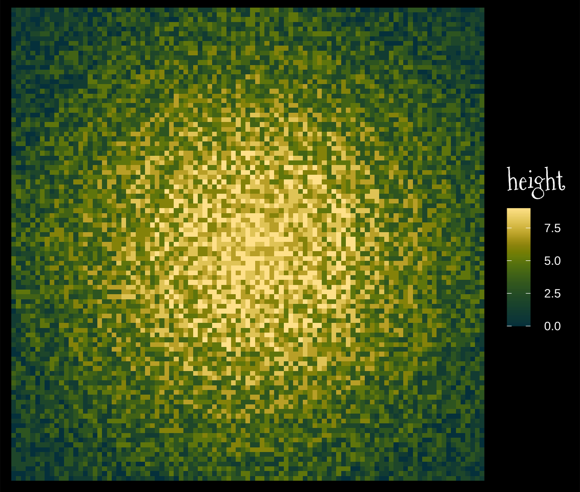
trees <- read_table("2022-12-8_assets/input.txt", col_names = F)

── Column specification ────────────────────────────────────────────────────────
cols(
  X1 = col_character()
)

trees |>
  pull(X1)|>
  map(~str_split(.x, pattern = "", simplify = T)) |>
  map(as.numeric) |>
  reduce(rbind) -> tree_mat
rownames(tree_mat) <- NULL

tree_mat |>
  data.frame() |>
  mutate(y = 1:n()) |>
  pivot_longer(-y, names_to = "x") |>
  mutate(x = str_remove(x, "X") |> as.numeric()) |>
  ggplot(aes(x, y, fill = value))+
    geom_raster() +
    scale_y_reverse(expand = expansion(mult = 0))+
    scale_x_continuous(expand = expansion(mult = 0))+
    scale_fill_bamako(reverse = FALSE)+
    labs(fill = "height")+
    coord_fixed()

Figure 1: Tree Height Map

I think if I was cleverer I could use some kind of convolution…

grad_max <- function(x, dir = 1){
  if(dir == 1){
    map(1:length(x), ~max(x[1:.x])) |>
      simplify() -> out
  }else{
    map(1:length(x), ~max(x[.x:length(x)])) |>
      simplify() -> out
  }
  return(out)
}

rev_diff <- function(x){
  out <- x |> rev() |> diff() |> rev()
  return(out)
}

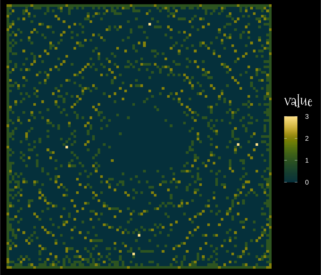
l_to_r <- apply(tree_mat, 1, grad_max) |> t()
r_to_l <- apply(tree_mat, 1, grad_max, dir = -1) |> t()
t_to_b <- apply(tree_mat, 2, grad_max)
b_to_t <- apply(tree_mat, 2, grad_max, dir = -1)

Ok, I spend a lot of time over thinking this. The visible trees are visible wherever this increasing max goes up. I’ll work that out for all 4 matrices (1 where visible, 0 otherwise) and just add them together. Any location >0 will be visible.

lr_vis <- apply(l_to_r, 1, diff) |> t()
lr_vis <- (lr_vis > 0)*1
lr_vis <- cbind(rep(1, 99), lr_vis)

rl_vis <- apply(r_to_l, 1, rev_diff) |> t()
rl_vis <- (rl_vis > 0)*1
rl_vis <- cbind(rl_vis, rep(1, 99))

tb_vis <- apply(t_to_b, 2, diff)
tb_vis <- (tb_vis > 0)*1
tb_vis <- rbind(rep(1, 99), tb_vis)

bt_vis <- apply(b_to_t, 2, rev_diff)
bt_vis <- (bt_vis > 0)*1
bt_vis <- rbind(bt_vis, rep(1, 99))

all_viz = lr_vis + rl_vis + bt_vis + tb_vis

all_viz |>
  data.frame() |>
  mutate(y = 1:n()) |>
  pivot_longer(-y, names_to = "x") |>
  mutate(x = str_remove(x, "X") |> as.numeric()) |>
  ggplot(aes(x, y, fill = value))+
    geom_raster() +
    scale_y_reverse(expand = expansion(mult = 0))+
    scale_x_continuous(expand = expansion(mult = 0))+
    scale_fill_bamako()+
    coord_fixed()

sum(all_viz > 0)

[1] 1801

Part 2

view_line_score <- function(x){
  score <- which((x - x[1])[-1] >= 0)[1]
  if(is.na(score)){
    return(length(x)-1)
  }else{
    return(score)
  }
}
scorer <- function(x, y, mat){
  view_line <- list(
    north = rev(mat[1:(x),y]),
    east = mat[x, (y):ncol(mat)],
    south = mat[x:nrow(mat), y],
    west = rev(mat[x, 1:y])
  )
  
  score <- 
  view_line |>
    map(view_line_score) |>
    reduce(`*`)

  return(score)
}

scorer(2,2, tree_mat)

[1] 4

expand_grid(
  x = 2:98,
  y = 2:98
) |>
  mutate(view_score = map2(x, y, ~scorer(.x, .y, tree_mat)) |> simplify()) -> view_scores

view_scores |>
  arrange(desc(view_score)) |>
  slice(1) -> winner
winner

# A tibble: 1 × 3
      x     y view_score
  <int> <int>      <dbl>
1    54    23     209880

view_scores |>
  ggplot(aes(x, y, fill = view_score))+
    geom_raster()+
    geom_text(data = winner, 
                 label = emoji("evergreen_tree"),
                 family = "Noto Emoji",
                 size = 10)+
    scale_fill_bamako(trans = "log10")+
    scale_y_reverse(expand = expansion(mult = 0))+
    scale_x_continuous(expand = expansion(mult = 0))+
    coord_fixed()  

Figure 2: Location of winning treehouse tree